实验三 数据分组、可视化与时间序列实验

一、实验要求

按要求完成题目，在实验报告中应有代码和运行截图以及心得体会

二、实验题目

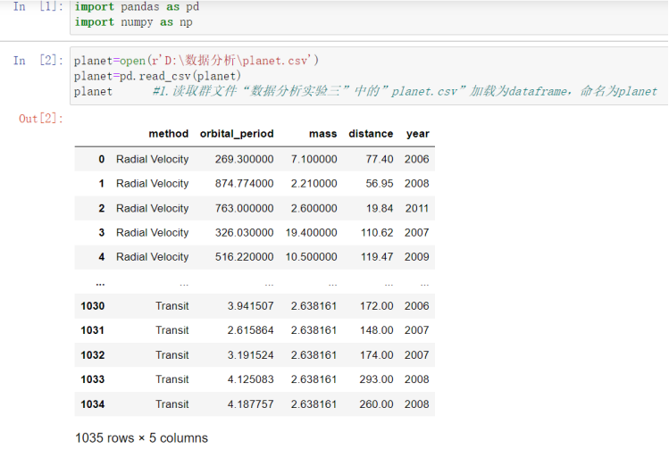
1 读取群文件“数据分析实验三”中的”planet.csv”加载为dataframe，命名为planet

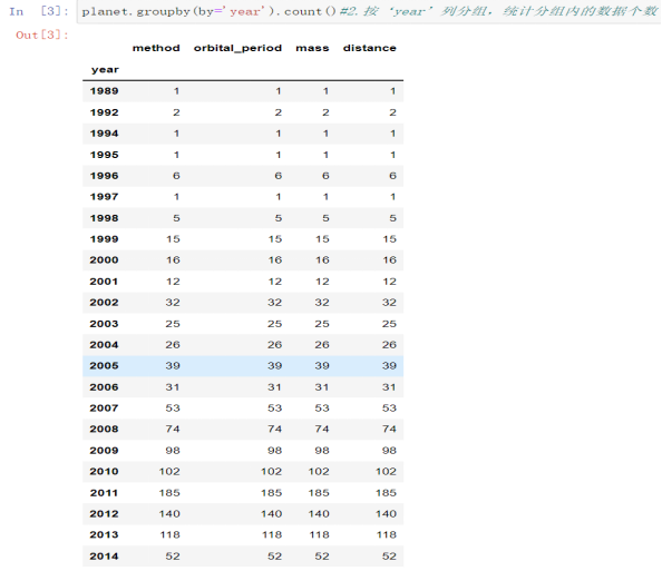
2 按‘year’列分组，统计分组内的数据个数

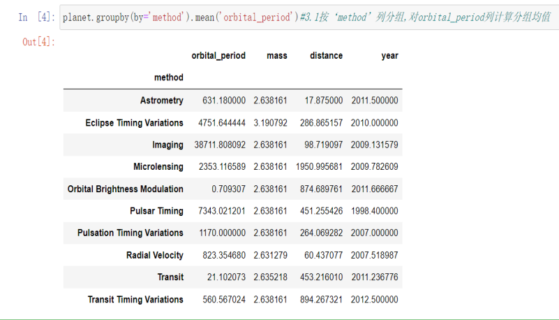
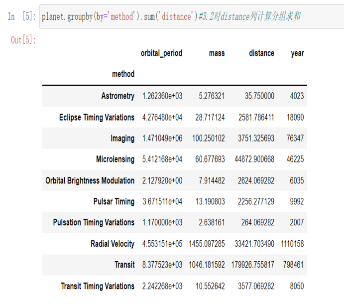
3 按‘method’列分组，对orbital_period列计算分组均值，对distance列计算分组求和

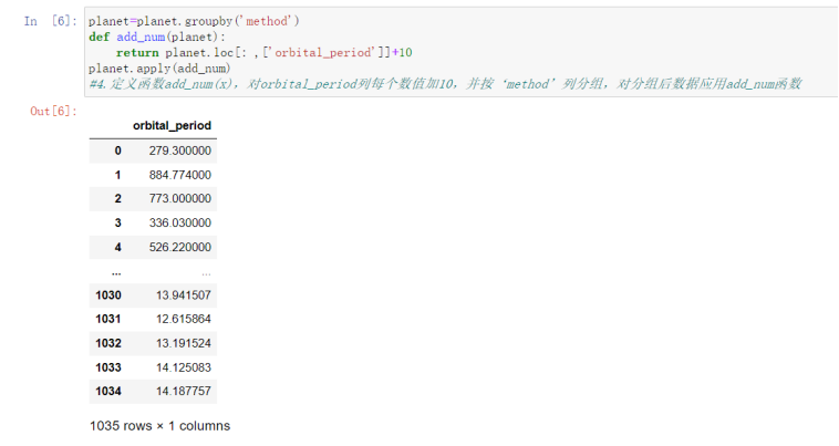
4 定义函数add_num(x)，对orbital_period列每个数值加10，并按‘method’列分组，对分组后数据应用add_num函数

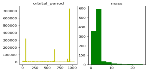
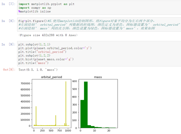
5 使用matplotlib绘制图形，将figure对象平均分为左右两个部分，左面绘制’ orbital_period’列数据的折线图，颜色定义为黄色，图标题设置为’ orbital_period’，右面绘制’ mass’列的直方图，颜色设置为绿色，图标题设置为’mass’，效果如图

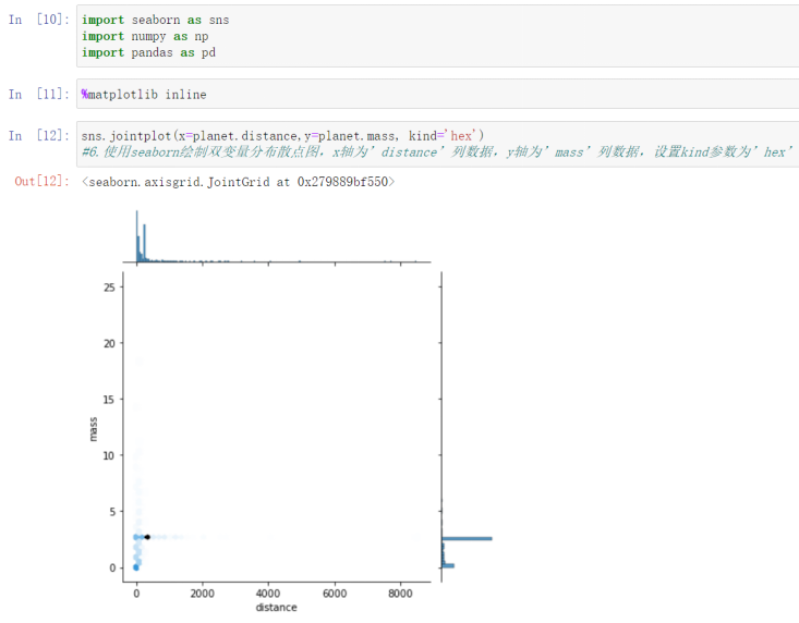
6 使用seaborn绘制双变量分布散点图，x轴为’distance’列数据，y轴为’mass’列数据，设置kind参数为’hex’

7 使用seaborn绘制distance列的直方图，设置bins=50

8 使用seaborn绘制条形图，x轴为’method’列数据，y轴为’distance’列数据

9 创建固定频率的DateIndex数据，从’20200101’号开始，频率为小时，长度为1035，命名为time_index

10 将time_index设置为planet的行索引

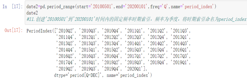
11 创建'20100501'到'20200101'时间内的固定频率时期索引，频率为季度，将时期索引命名为period_index

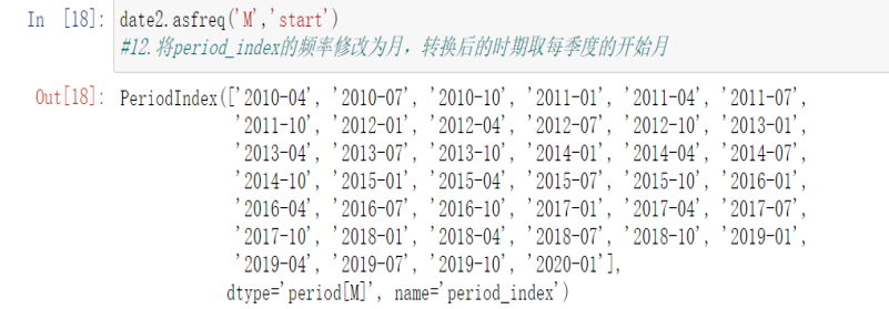
12 将period_index的频率修改为月，转换后的时期取每季度的开始月

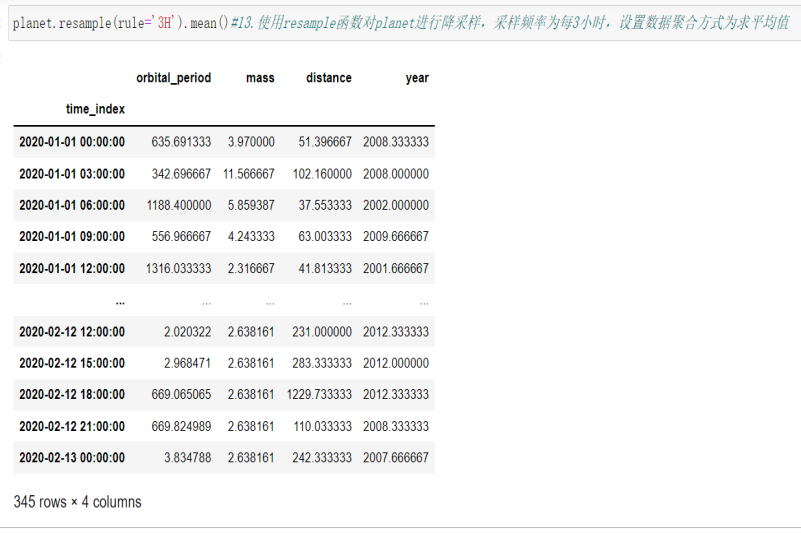
13 使用resample函数对planet进行降采样，采样频率为每3小时，设置数据聚合方式为求平均值

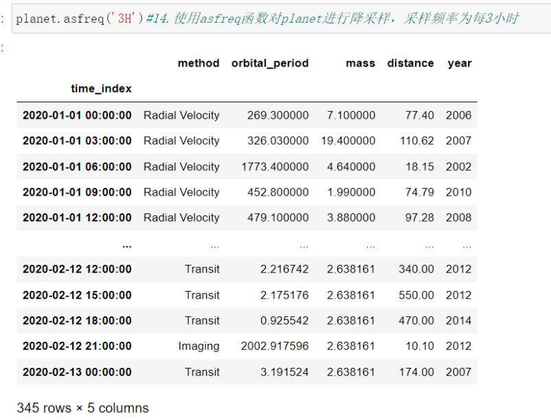
14 使用asfreq函数对planet进行降采样，采样频率为每3小时

15 使用resample函数对planet进行升采样，采样频率为每30分钟，将缺失值填充为你的学号

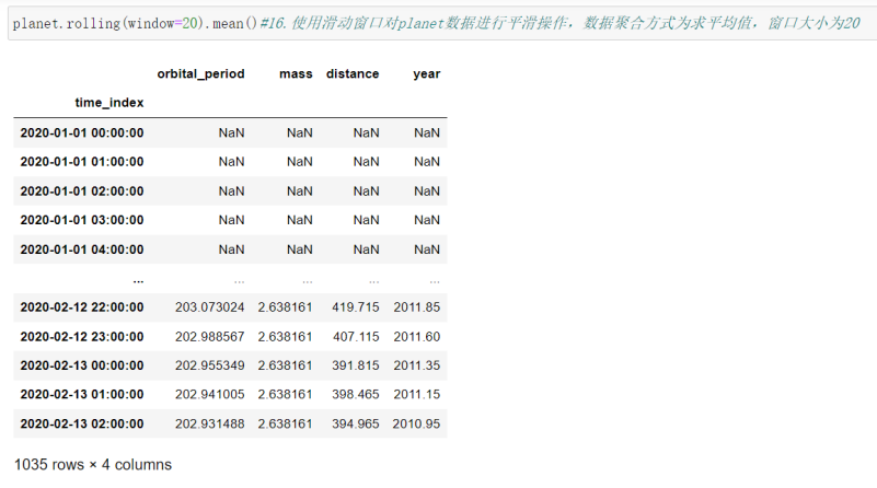
16 使用滑动窗口对planet数据进行平滑操作，数据聚合方式为求平均值，窗口大小为20

 

三、实验代码与运行结果：

 

  1.  import pandas as pd

 

import numpy as np

 

planet=open(r'D:\数据分析\planet.csv')

 

planet=pd.read_csv(planet)

 

planet   #读取群文件“数据分析实验三”中的”planet.csv”加载为dataframe

2. planet.groupby(by='year').count()   #按‘year’列分组，统计分组内的数据个数

3.  planet.groupby(by='method').mean('orbital_period')

 

#3.1按‘method’列分组,对orbital_period列计算分组均值

 

 

 planet.groupby(by='method').sum('distance')

#3.2对distance列计算分组求和

4.  planet=planet.groupby('method')

 

def add_num(planet):

 

    return planet.loc[: ,['orbital_period']]+10

 

planet.apply(add_num)

 

#定义函数add_num(x)，对orbital_period列每个数值加10，并按‘method’列分组，对分组后数据应用add_num函数

 

 

 

5.         import matplotlib.pyplot as plt

import numpy as np

%matplotlib inline

 fig=plt.figure()

#使用matplotlib绘制图形，将figure对象平均分为左右两个部分，

#左面绘制’ orbital_period’列数据的折线图，颜色定义为黄色，图标题设置为 ’ orbital_period’

#右面绘制’ mass’列的直方图，颜色设置为绿色，图标题设置为’mass’，效果如图

 plt.subplot(1,2,1)

plt.plot(planet.orbital_period,color='y')

plt.title("orbital_period")

plt.subplot(1,2,2)

plt.hist(planet.mass,color='g')

plt.title("mass")

 

 6.     import seaborn as sns

import numpy as np

import pandas as pd

%matplotlib inline

sns.jointplot(x=planet.distance,y=planet.mass, kind='hex')

#使用seaborn绘制双变量分布散点图，x轴为’distance’列数据，y轴为’mass’列数据，设置kind参数为’hex’

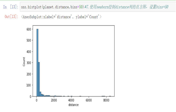
7.        sns.histplot(planet.distance,bins=50)

  #使用seaborn绘制distance列的直方图，设置bins=50

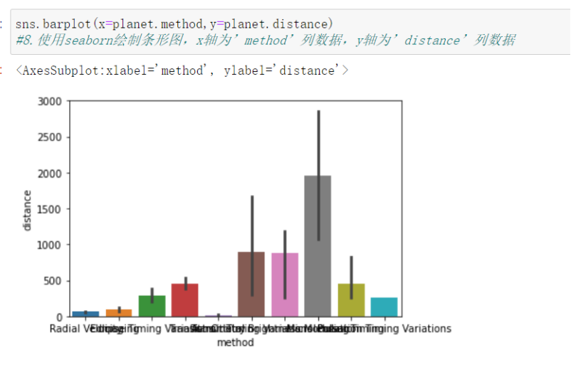
8.sns.barplot(x=planet.method,y=planet.distance)

#使用seaborn绘制条形图，x轴为’method’列数据，y轴为’distance’列数据

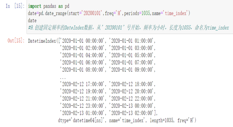
9. import pandas as pd

  date=pd.date_range(start='20200101',freq='H',periods=1035,name='time_index')

  date

#创建固定频率的DateIndex数据，从’20200101’号开始，频率为小时，长度为1035，命名为time_index

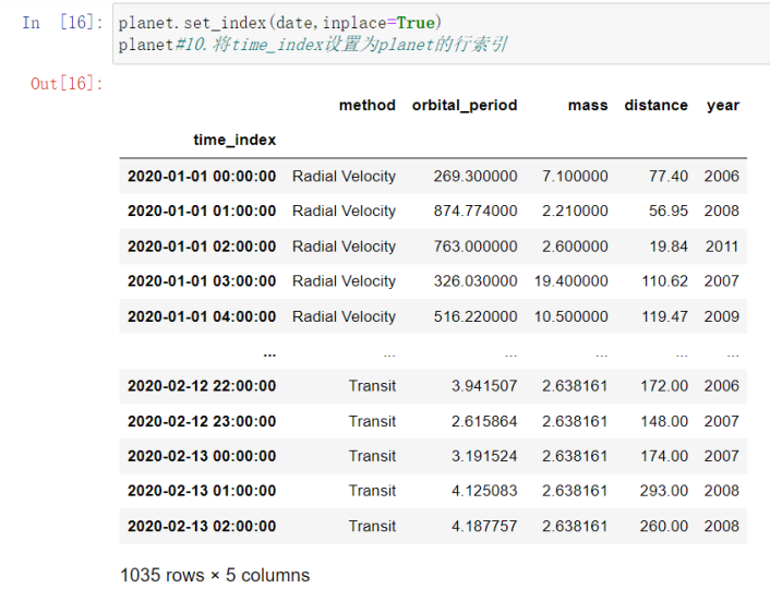
10 planet.set_index(date,inplace=True)  

   planet    #将time_index设置为planet的行索引

 

 

 11date2=pd.period_range(start='20100501',end='20200101',freq='Q',name='period_index')

     date2   #创建'20100501'到'20200101'时间内的固定频率时期索引，频率为季度，将时期索引命名为period_index

12 date2.asfreq('M','start')

#将period_index的频率修改为月，转换后的时期取每季度的开始月

13 planet.resample(rule='3H').mean()#使用resample函数对planet进行降采样，采样频率为每3小时，设置数据聚合方式为求平均值

 

 

 14 planet.asfreq('3H')#使用asfreq函数对planet进行降采样，采样频率为每3小时

 

 

 

15 planet.resample('30min').asfreq(fill_value=’xxxxx’)

#使用resample函数对planet进行升采样，采样频率为每30分钟，将缺失值填充为你的学号

（截图自己实现）

16 planet.rolling(window=20).mean()#16.使用滑动窗口对planet数据进行平滑操作，数据聚合方式为求平均值，窗口大小为20