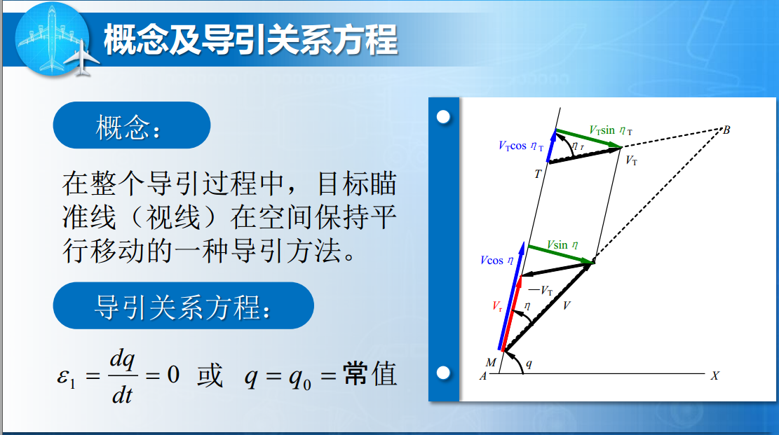
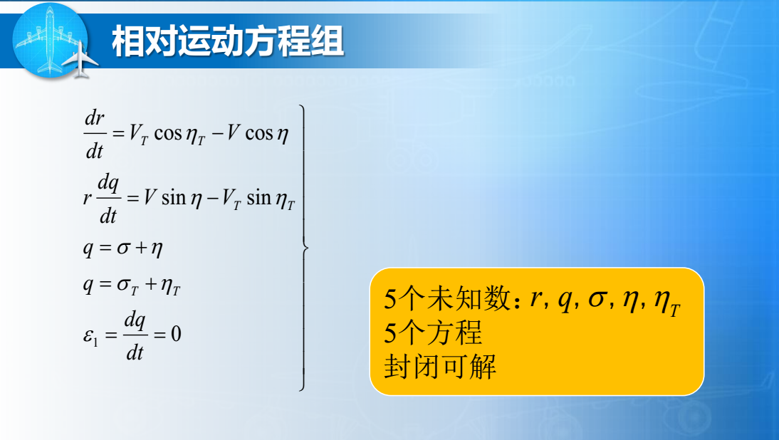
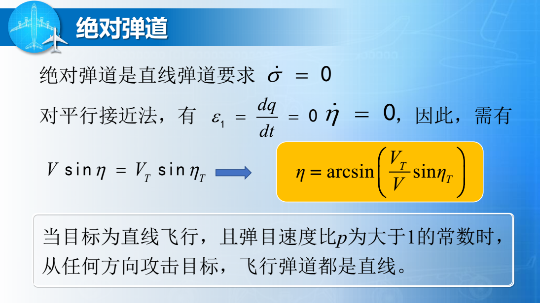
平行接近法导引弹道仿真

代码：

点击查看python代码

import numpy as np
from math import *
import matplotlib.pyplot as plt
plt.rcParams ['font.sans-serif']= ['SimHei'] 

def PingXing():
    xM = 0*1000
    yM = 0*1000
    #初始弹道倾角
    gammaM = 240/57.3
    Vm = 300
    aM = 10
    xT = 5*1000
    yT = 5*1000
    #初始弹道倾角
    gammaT = 5/57.3
    Vt = 300
    aT = 0

    T = 100
    step = 0.001
    K = int(T/step)
    pM = []
    pT = []
    gammaMA = []
    tn = []
    for i in range(0,K):
        #目标运动方程
        dVt = aT
        gammaT += (0.2*step)/57.3;
        Vt  = Vt + step*dVt
        dxT = Vt*cos(gammaT)
        dyT = Vt*sin(gammaT)
        xT  = xT + step*dxT
        yT  = yT + step*dyT

        #相对运动方程
        drx    = xT - xM
        dry    = yT - yM
        q      = atan2(dry,drx)
        yetaT  = q - gammaT             #目标速度矢量前置角
        yetaM  = asin(Vt/Vm*sin(yetaT)) #平行接近法制导律指令导弹速度矢量前置角
        gammaM = q-yetaM
        print('飞行时间 %6.3f ' % (i*step),
              '视线角q %6.3f' % (q*57.3),
              'yetaT %6.3f' % (yetaT*57.3),
              'yetaM %6.3f' % (yetaM*57.3))
        
        #导弹运动方程
        dVm = aM
        dxM = Vm*cos(gammaM)
        dyM = Vm*sin(gammaM)
        xM  = xM + step*dxM
        yM  = yM + step*dyM
        Vm  = Vm + step*dVm
        gammaMdot = aM/Vm
        gammaTdot = aT/Vt
        pM.append([xM,yM])
        pT.append([xT,yT])
        tn.append(i*step)
        gammaMA.append([gammaM*57.3])
        if((yT < 0) or (yM <0)):
            break;
        if(sqrt((yT-yM)**2 + (xT-xM)**2)<1):
            break;
    pM = np.array(pM)
    pT = np.array(pT)
    show_GT(pM,pT)
    show_Var(tn,gammaMA)
    

def show_Var(tn,Var):
    plt.scatter(tn,Var,s=1)
    plt.xlabel('x-price')
    plt.ylabel('y-amount')
    plt.legend(loc=4)  # 指定legend的位置,类似象限的位置
    plt.title('速度矢量前置角')
    plt.show()

def show_GT(pM,pT):
    plot2 = plt.plot(pM[:,0], pM[:,1], 'r', label='导弹运动轨迹')
    plot2 = plt.plot(pT[:,0], pT[:,1], 'b', label='目标运动轨迹')
    # plt.scatter(pM[:,0], pM[:,1],s=1, label='导弹运动轨迹')
    # plt.scatter(pT[:,0], pT[:,1],s=1, label='目标运动轨迹')
    plt.xlabel('x-price')
    plt.ylabel('y-amount')
    plt.legend(loc=4)  # 指定legend的位置,类似象限的位置
    plt.title('平行接近导引弹道')
    plt.show()
    #plt.savefig('polyfit.png')



if __name__ == "__main__":
    PingXing()

仿真结果：

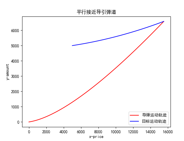
优点：弹道平直，末端过载较小
缺点：需要目标的速度及速度矢量前置角信息