7.4 NIN

 

7.4.0 头文件

import torch
from torch import nn
from d2l import torch as d2l
from matplotlib import pyplot as plt

 

7.4.1 NiN网络模型

# 创建一个NiN块，NiN块包含三个卷积层，第一个是自己指定卷积核尺寸的卷积层，后面两个是1×1卷积层
def nin_block(in_channels, out_channels, kernel_size, strides, padding):
    return nn.Sequential(
        nn.Conv2d(in_channels, out_channels, kernel_size, strides, padding),nn.ReLU(),  # 第一个卷积层，卷积核尺寸自己指定，和一个ReLU层
        nn.Conv2d(out_channels, out_channels, kernel_size=1), nn.ReLU(),                # 第二个卷积层，卷积核尺寸为1×1，1×1卷积核失去了卷积层识别相邻元素间相互作用的能力，但可以看作在每个像素位置应用的全连接层，能够将同一像素位置上的多个通道的输入值转换成多个通道的输出值，和一个ReLU层
        nn.Conv2d(out_channels, out_channels, kernel_size=1), nn.ReLU())                # 第二个卷积层，卷积核尺寸为1×1，1×1卷积核失去了卷积层识别相邻元素间相互作用的能力，但可以看作在每个像素位置应用的全连接层，能够将同一像素位置上的多个通道的输入值转换成多个通道的输出值，和一个ReLU层

# 定义NiN网络模型，NiN块→最大池化层→NiN块→最大池化层→NiN块→最大池化层→Dropout层→NiN块→全局最大池化层→展平层
net = nn.Sequential(
    nin_block(1, 96, kernel_size=11, strides=4, padding=0),
    nn.MaxPool2d(3, stride=2),
    nin_block(96, 256, kernel_size=5, strides=1, padding=2),
    nn.MaxPool2d(3, stride=2),
    nin_block(256, 384, kernel_size=3, strides=1, padding=1),
    nn.MaxPool2d(3, stride=2),
    nn.Dropout(0.5),
    # 标签类别数是10
    nin_block(384, 10, kernel_size=3, strides=1, padding=1),
    nn.AdaptiveAvgPool2d((1, 1)),
    # 将四维的输出转成二维的输出，其形状为(批量大小,10)
    nn.Flatten())

# 构建一个行和列都为224的单通道样本，观察每个VGG块、全连接层输出的形状

X = torch.rand(size=(1, 1, 224, 224))
for layer in net:
    X = layer(X)
    print(layer.__class__.__name__,'output shape:\t', X.shape)
# 输出：
# Sequential output shape:     torch.Size([1, 96, 54, 54])
# MaxPool2d output shape:     torch.Size([1, 96, 26, 26])
# Sequential output shape:     torch.Size([1, 256, 26, 26])
# MaxPool2d output shape:     torch.Size([1, 256, 12, 12])
# Sequential output shape:     torch.Size([1, 384, 12, 12])
# MaxPool2d output shape:     torch.Size([1, 384, 5, 5])
# Dropout output shape:     torch.Size([1, 384, 5, 5])
# Sequential output shape:     torch.Size([1, 10, 5, 5])
# AdaptiveAvgPool2d output shape:     torch.Size([1, 10, 1, 1])
# Flatten output shape:     torch.Size([1, 10])

 

7.4.2 训练过程

# 定义学习率、训练轮数、批量大小
lr, num_epochs, batch_size = 0.1, 10, 128
# 下载fashion_mnist，并对数据集进行打乱和按批量大小进行切割的操作，得到可迭代的训练集和测试集（训练集和测试集的形式都为（特征数据集合，数字标签集合））,同时将图像从28×28放大为224×224
train_iter, test_iter = d2l.load_data_fashion_mnist(batch_size, resize=224)
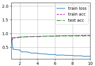
# 使用GPU对模型进行训练，输出最后一轮训练时的平均损失、在训练集上的平均准确率、在测试集上的平均准测率，输出每秒能够训练多少张图像
d2l.train_ch6(net, train_iter, test_iter, num_epochs, lr, d2l.try_gpu())
# 输出：
# loss 2.303, train acc 0.100, test acc 0.100
# 91.3 examples/sec on cuda:0

 

7.4.2 训练结果可视化

plt.savefig('OutPut.png')

 

 

本小节完整代码如下

import torch
from torch import nn
from d2l import torch as d2l
from matplotlib import pyplot as plt

# ------------------------------NiN网络模型------------------------------------

# 创建一个NiN块，NiN块包含三个卷积层，第一个是自己指定卷积核尺寸的卷积层，后面两个是1×1卷积层
def nin_block(in_channels, out_channels, kernel_size, strides, padding):
    return nn.Sequential(
        nn.Conv2d(in_channels, out_channels, kernel_size, strides, padding),nn.ReLU(),  # 第一个卷积层，卷积核尺寸自己指定，和一个ReLU层
        nn.Conv2d(out_channels, out_channels, kernel_size=1), nn.ReLU(),                # 第二个卷积层，卷积核尺寸为1×1，1×1卷积核失去了卷积层识别相邻元素间相互作用的能力，但可以看作在每个像素位置应用的全连接层，能够将同一像素位置上的多个通道的输入值转换成多个通道的输出值，和一个ReLU层
        nn.Conv2d(out_channels, out_channels, kernel_size=1), nn.ReLU())                # 第二个卷积层，卷积核尺寸为1×1，1×1卷积核失去了卷积层识别相邻元素间相互作用的能力，但可以看作在每个像素位置应用的全连接层，能够将同一像素位置上的多个通道的输入值转换成多个通道的输出值，和一个ReLU层

# 定义NiN网络模型，NiN块→最大池化层→NiN块→最大池化层→NiN块→最大池化层→Dropout层→NiN块→全局最大池化层→展平层
net = nn.Sequential(
    nin_block(1, 96, kernel_size=11, strides=4, padding=0),
    nn.MaxPool2d(3, stride=2),
    nin_block(96, 256, kernel_size=5, strides=1, padding=2),
    nn.MaxPool2d(3, stride=2),
    nin_block(256, 384, kernel_size=3, strides=1, padding=1),
    nn.MaxPool2d(3, stride=2),
    nn.Dropout(0.5),
    # 标签类别数是10
    nin_block(384, 10, kernel_size=3, strides=1, padding=1),
    nn.AdaptiveAvgPool2d((1, 1)),
    # 将四维的输出转成二维的输出，其形状为(批量大小,10)
    nn.Flatten())

# 构建一个行和列都为224的单通道样本，观察每个VGG块、全连接层输出的形状
X = torch.rand(size=(1, 1, 224, 224))
for layer in net:
    X = layer(X)
    print(layer.__class__.__name__,'output shape:\t', X.shape)
# 输出：
# Sequential output shape:     torch.Size([1, 96, 54, 54])
# MaxPool2d output shape:     torch.Size([1, 96, 26, 26])
# Sequential output shape:     torch.Size([1, 256, 26, 26])
# MaxPool2d output shape:     torch.Size([1, 256, 12, 12])
# Sequential output shape:     torch.Size([1, 384, 12, 12])
# MaxPool2d output shape:     torch.Size([1, 384, 5, 5])
# Dropout output shape:     torch.Size([1, 384, 5, 5])
# Sequential output shape:     torch.Size([1, 10, 5, 5])
# AdaptiveAvgPool2d output shape:     torch.Size([1, 10, 1, 1])
# Flatten output shape:     torch.Size([1, 10])

# ------------------------------训练过程------------------------------------

# 定义学习率、训练轮数、批量大小
lr, num_epochs, batch_size = 0.1, 10, 128
# 下载fashion_mnist，并对数据集进行打乱和按批量大小进行切割的操作，得到可迭代的训练集和测试集（训练集和测试集的形式都为（特征数据集合，数字标签集合））,同时将图像从28×28放大为224×224
train_iter, test_iter = d2l.load_data_fashion_mnist(batch_size, resize=224)
# 使用GPU对模型进行训练，输出最后一轮训练时的平均损失、在训练集上的平均准确率、在测试集上的平均准测率，输出每秒能够训练多少张图像
d2l.train_ch6(net, train_iter, test_iter, num_epochs, lr, d2l.try_gpu())
# 输出：
# loss 2.303, train acc 0.100, test acc 0.100
# 91.3 examples/sec on cuda:0

# ------------------------------训练结果可视化------------------------------------

plt.savefig('OutPut.png')