4.4 欠拟合与过拟合

 

4.4.0 头文件

 

import math
import numpy as np
import torch
from torch import nn
from d2l import torch as d2l
from matplotlib import pyplot as plt

 

4.4.1利用三阶多项式来制作数据集

 

# 设置训练集大小和测试集大小
n_train, n_test = 100, 100
# 设置允许的多项式最大阶数（0~19阶），即数据的输入特征最多有20个特征
max_degree = 20

# 设置真实的权重w
true_w = np.zeros(max_degree)
true_w[0:4] = np.array([5, 1.2, -3.4, 5.6]) #按照公式，只设置0~3阶的权重，其他的权重都为零

# 随机生成200个样本x，并将200个样本打乱
features = np.random.normal(size=(n_train + n_test, 1))
np.random.shuffle(features)

# 计算出每隔样本的所有输入特征（包括阶乘）
poly_features = np.power(features, np.arange(max_degree).reshape(1, -1))
for i in range(max_degree):
    poly_features[:, i] /= math.gamma(i + 1)  # gamma(n)=(n-1)!

# 计算每个样本的真实标签，需要加上噪声
labels = np.dot(poly_features, true_w)
labels += np.random.normal(scale=0.1, size=labels.shape)

# 将真实权重, 样本x, 输入特征, 真实标签转换成张量
true_w, features, poly_features, labels = [torch.tensor(x, dtype=torch.float32) for x in [true_w, features, poly_features, labels]]

 

 

 

4.4.2 计算网络模型在训练集或数据集上的损失均值

 

# net：定义的网络模型
# data_iter：打乱的并且根据批量大小切割好的训练集或测试集
# loss：损失函数
# 计算网络模型在训练集或数据集上的损失均值
def evaluate_loss(net, data_iter, loss):
    metric = d2l.Accumulator(2)  #网络模型在训练集或数据集上的损失总和,训练集或测试集的样本总量
    for X, y in data_iter:
        # 计算一个批量的预测值
        out = net(X)
        y = y.reshape(out.shape)
        # 计算一个批量的损失
        l = loss(out, y)
        # 将网络模型在训练集或数据集上的损失总和 和 训练集或测试集的样本总量 两个变量累加
        metric.add(l.sum(), l.numel())
    # 返回网络模型在训练集或数据集上的损失均值
    return metric[0] / metric[1]

 

 

 

4.4.3 训练过程

 

def train(train_features, test_features, train_labels, test_labels,num_epochs=400):
    # 定义均方误差损失函数，得到每个样本的损失
    loss = nn.MSELoss(reduction='none')
    input_shape = train_features.shape[-1]  #训练集一个100个样本，每个样本有input_shape个输入特征
    # 定义网络模型，网络模型中只有一个全连接层，全连接层input_shape个输入，一个输出，不设置偏移量，因为input_shape个特征中有一个特征对应的是偏移量
    net = nn.Sequential(nn.Linear(input_shape, 1, bias=False))
    # 设置批量大小为10
    batch_size = min(10, train_labels.shape[0])
    # 获取经过按照批量大小进行切割和封装过的训练集，可迭代读取，每次迭代读取出一个批量的数据（特征 + 对应的标签）
    train_iter = d2l.load_array((train_features, train_labels.reshape(-1,1)), batch_size)
    # 获取经过按照批量大小进行切割和封装过的测试集，可迭代读取，每次迭代读取出一个批量的数据（特征 + 对应的标签）
    test_iter = d2l.load_array((test_features, test_labels.reshape(-1,1)),batch_size, is_train=False)
    # 定义优化器
    trainer = torch.optim.SGD(net.parameters(), lr=0.01)
    # 定义动画，显示训练结果
    animator = d2l.Animator(xlabel='epoch', ylabel='loss', yscale='log',xlim=[1, num_epochs], ylim=[1e-3, 1e2],legend=['train', 'test'])

    # 进行400轮训练
    for epoch in range(num_epochs):
        # 进行一轮训练
        d2l.train_epoch_ch3(net, train_iter, loss, trainer)
        # 每隔20轮，将训练得到的模型在训练集和测试集上分别计算一次损失（训练损失、泛化损失）
        if epoch == 0 or (epoch + 1) % 20 == 0:
            animator.add(epoch + 1, (evaluate_loss(net, train_iter, loss),evaluate_loss(net, test_iter, loss)))
    # 输出训练得到的模型权重
    print('weight:', net[0].weight.data.numpy())

# 用三阶多项式来拟合模型（正常）
# poly_features[:n_train, :4]：将前100个样本在每个阶数的特征值作为训练集（用三阶来拟合，所以只取前4个特征）
# poly_features[n_train:, :4]：将后100个样本在每个阶数的特征值作为训练集（用三阶来拟合，所以只取前4个特征）
# labels[:n_train]：将前100个样本的输出值作为训练集标签
# labels[n_train:]：将后100个样本的输出值作为测试集标签
train(poly_features[:n_train, :4], poly_features[n_train:, :4],labels[:n_train], labels[n_train:])
# 输出：
# weight: [[ 5.015506   1.2249223 -3.3873422  5.5354605]]

# 用一阶多项式来拟合模型（欠拟合）
# poly_features[:n_train, :2]：将前100个样本在每个阶数的特征值作为训练集（用一阶来拟合，所以只取前2个特征）
# poly_features[n_train:, :2]：将后100个样本在每个阶数的特征值作为训练集（用一阶来拟合，所以只取前2个特征）
# labels[:n_train]：将前100个样本的输出值作为训练集标签
# labels[n_train:]：将后100个样本的输出值作为测试集标签train(poly_features[:n_train, :2], poly_features[n_train:, :2],labels[:n_train], labels[n_train:])
# 输出：
# weight: [[3.4878697 3.5113552]]

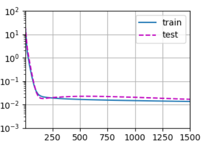
# 用十九阶多项式来拟合模型（过拟合）
# poly_features[:n_train, :]：将前100个样本在每个阶数的特征值作为训练集（用十九阶来拟合，所以取前20个特征）
# poly_features[n_train:, :]：将后100个样本在每个阶数的特征值作为训练集（用十九阶来拟合，所以只取前20个特征）
# labels[:n_train]：将前100个样本的输出值作为训练集标签
# labels[n_train:]：将后100个样本的输出值作为测试集标签train(poly_features[:n_train, :], poly_features[n_train:, :],labels[:n_train], labels[n_train:], num_epochs=1500)
# 输出：
# weight: [[ 4.99926233e+00  1.25115871e+00 -3.30954051e+00  5.25334406e+00
#   -1.84362158e-01  1.19941306e+00 -1.35312080e-01  3.56987506e-01
#   -4.66701621e-03 -2.12772131e-01 -3.00819799e-02  2.23305166e-01
#   -1.01899929e-01 -2.07265347e-01  2.22946733e-01 -1.81735992e-01
#   -1.20312020e-01  1.53819770e-01 -1.10108346e-01  1.31270021e-01]]

 

 

 

 

本小节完整代码如下所示

import math
import numpy as np
import torch
from torch import nn
from d2l import torch as d2l
from matplotlib import pyplot as plt

# ------------------------------利用三阶多项式来制作数据集------------------------------------

# 设置训练集大小和测试集大小
n_train, n_test = 100, 100
# 设置允许的多项式最大阶数（0~19阶），即数据的输入特征最多有20个特征
max_degree = 20

# 设置真实的权重w
true_w = np.zeros(max_degree)
true_w[0:4] = np.array([5, 1.2, -3.4, 5.6]) #按照公式，只设置0~3阶的权重，其他的权重都为零

# 随机生成200个样本x，并将200个样本打乱
features = np.random.normal(size=(n_train + n_test, 1))
np.random.shuffle(features)

# 计算出每隔样本的所有输入特征（包括阶乘）
poly_features = np.power(features, np.arange(max_degree).reshape(1, -1))
for i in range(max_degree):
    poly_features[:, i] /= math.gamma(i + 1)  # gamma(n)=(n-1)!

# 计算每个样本的真实标签，需要加上噪声
labels = np.dot(poly_features, true_w)
labels += np.random.normal(scale=0.1, size=labels.shape)

# 将真实权重, 样本x, 输入特征, 真实标签转换成张量
true_w, features, poly_features, labels = [torch.tensor(x, dtype=torch.float32) for x in [true_w, features, poly_features, labels]]

# ------------------------------计算网络模型在训练集或数据集上的损失均值------------------------------------

# net：定义的网络模型
# data_iter：打乱的并且根据批量大小切割好的训练集或测试集
# loss：损失函数
# 计算网络模型在训练集或数据集上的损失均值
def evaluate_loss(net, data_iter, loss):
    metric = d2l.Accumulator(2)  #网络模型在训练集或数据集上的损失总和,训练集或测试集的样本总量
    for X, y in data_iter:
        # 计算一个批量的预测值
        out = net(X)
        y = y.reshape(out.shape)
        # 计算一个批量的损失
        l = loss(out, y)
        # 将网络模型在训练集或数据集上的损失总和 和 训练集或测试集的样本总量 两个变量累加
        metric.add(l.sum(), l.numel())
    # 返回网络模型在训练集或数据集上的损失均值
    return metric[0] / metric[1]

# ------------------------------训练过程------------------------------------

def train(train_features, test_features, train_labels, test_labels,num_epochs=400):
    # 定义均方误差损失函数，得到每个样本的损失
    loss = nn.MSELoss(reduction='none')
    input_shape = train_features.shape[-1]  #训练集一个100个样本，每个样本有input_shape个输入特征
    # 定义网络模型，网络模型中只有一个全连接层，全连接层input_shape个输入，一个输出，不设置偏移量，因为input_shape个特征中有一个特征对应的是偏移量
    net = nn.Sequential(nn.Linear(input_shape, 1, bias=False))
    # 设置批量大小为10
    batch_size = min(10, train_labels.shape[0])
    # 获取经过按照批量大小进行切割和封装过的训练集，可迭代读取，每次迭代读取出一个批量的数据（特征 + 对应的标签）
    train_iter = d2l.load_array((train_features, train_labels.reshape(-1,1)), batch_size)
    # 获取经过按照批量大小进行切割和封装过的测试集，可迭代读取，每次迭代读取出一个批量的数据（特征 + 对应的标签）
    test_iter = d2l.load_array((test_features, test_labels.reshape(-1,1)),batch_size, is_train=False)
    # 定义优化器
    trainer = torch.optim.SGD(net.parameters(), lr=0.01)
    # 定义动画，显示训练结果
    animator = d2l.Animator(xlabel='epoch', ylabel='loss', yscale='log',xlim=[1, num_epochs], ylim=[1e-3, 1e2],legend=['train', 'test'])

    # 进行400轮训练
    for epoch in range(num_epochs):
        # 进行一轮训练
        d2l.train_epoch_ch3(net, train_iter, loss, trainer)
        # 每隔20轮，将训练得到的模型在训练集和测试集上分别计算一次损失（训练损失、泛化损失）
        if epoch == 0 or (epoch + 1) % 20 == 0:
            animator.add(epoch + 1, (evaluate_loss(net, train_iter, loss),evaluate_loss(net, test_iter, loss)))
    # 输出训练得到的模型权重
    print('weight:', net[0].weight.data.numpy())

# 用三阶多项式来拟合模型（正常）
# poly_features[:n_train, :4]：将前100个样本在每个阶数的特征值作为训练集（用三阶来拟合，所以只取前4个特征）
# poly_features[n_train:, :4]：将后100个样本在每个阶数的特征值作为训练集（用三阶来拟合，所以只取前4个特征）
# labels[:n_train]：将前100个样本的输出值作为训练集标签
# labels[n_train:]：将后100个样本的输出值作为测试集标签
# train(poly_features[:n_train, :4], poly_features[n_train:, :4],labels[:n_train], labels[n_train:])
# 输出：
# weight: [[ 5.015506   1.2249223 -3.3873422  5.5354605]]

# 用一阶多项式来拟合模型（欠拟合）
# poly_features[:n_train, :2]：将前100个样本在每个阶数的特征值作为训练集（用一阶来拟合，所以只取前2个特征）
# poly_features[n_train:, :2]：将后100个样本在每个阶数的特征值作为训练集（用一阶来拟合，所以只取前2个特征）
# labels[:n_train]：将前100个样本的输出值作为训练集标签
# labels[n_train:]：将后100个样本的输出值作为测试集标签
# train(poly_features[:n_train, :2], poly_features[n_train:, :2],labels[:n_train], labels[n_train:])
# 输出：
# weight: [[3.4878697 3.5113552]]

# 用十九阶多项式来拟合模型（过拟合）
# poly_features[:n_train, :]：将前100个样本在每个阶数的特征值作为训练集（用十九阶来拟合，所以取前20个特征）
# poly_features[n_train:, :]：将后100个样本在每个阶数的特征值作为训练集（用十九阶来拟合，所以只取前20个特征）
# labels[:n_train]：将前100个样本的输出值作为训练集标签
# labels[n_train:]：将后100个样本的输出值作为测试集标签
train(poly_features[:n_train, :], poly_features[n_train:, :],labels[:n_train], labels[n_train:], num_epochs=1500)
# 输出：
# weight: [[ 4.99926233e+00  1.25115871e+00 -3.30954051e+00  5.25334406e+00
#   -1.84362158e-01  1.19941306e+00 -1.35312080e-01  3.56987506e-01
#   -4.66701621e-03 -2.12772131e-01 -3.00819799e-02  2.23305166e-01
#   -1.01899929e-01 -2.07265347e-01  2.22946733e-01 -1.81735992e-01
#   -1.20312020e-01  1.53819770e-01 -1.10108346e-01  1.31270021e-01]]

# ------------------------------训练结果可视化------------------------------------

plt.savefig('Output.png')