图Lasso求逆协方差矩阵(Graphical Lasso for inverse covariance matrix)

作者：凯鲁嘎吉 - 博客园 http://www.cnblogs.com/kailugaji/

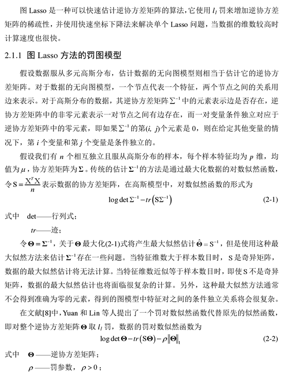
1. 图Lasso方法的基本理论

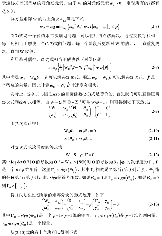
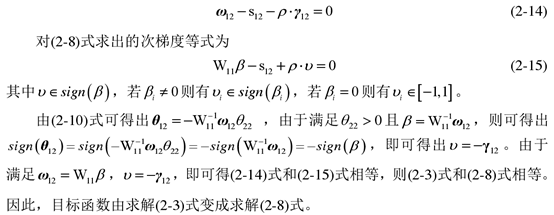
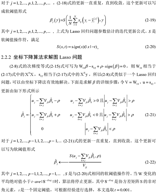
2. 坐标下降算法

3. 图Lasso算法

4. MATLAB程序

数据见参考文献[2]

4.1 方法一

demo.m

load SP500
data = normlization(data);
S = cov(data);  %样本协方差
[X, W] = glasso_1(double(S), 0.5);
%X:sigma^(-1), W:sigma
[~, idx] = sort(info(:,3));
colormap gray
imagesc(X(idx, idx) == 0)
axis off
 
%% Data Normalization
function data = normlization(data)
data = bsxfun(@minus, data, mean(data));
data = bsxfun(@rdivide, data, std(data));
end

glasso_1.m

function [X, W] = glasso_1(S, lambda)
%% Graphical Lasso - Friedman et. al, Biostatistics, 2008
% Input:
%   S - 样本的协方差矩阵
%   lambda - 罚参数
% Output:
%   X - 精度矩阵    sigma^(-1)
%   W - 协方差矩阵   sigma
%%
p = size(S,1);  %数据维度
W = S + lambda * eye(p);  %W=S+λI
beta = zeros(p) - lambda * eye(p);   %β=-λI
eps = 1e-4;
finished = false(p);   %finished:p*p的逻辑0矩阵
while true
    for j = 1 : p
        idx = 1 : p; idx(j) = [];
        beta(idx, j) = lasso(W(idx, idx), S(idx, j), lambda, beta(idx, j));
        W(idx, j) = W(idx,idx) * beta(idx, j);  %W=W*β
        W(j, idx) = W(idx, j);
    end
    index = (beta == 0);
    finished(index) = (abs(W(index) - S(index)) <= lambda);
    finished(~index) = (abs(W(~index) -S(~index) + lambda * sign(beta(~index))) < eps);
    if finished
        break;
    end
end
X = zeros(p);
for j = 1 : p
    idx = 1 : p; idx(j) = [];
    X(j,j) = 1 / (W(j,j) - dot(W(idx,j), beta(idx,j)));
    X(idx, j) = -1 * X(j, j) * beta(idx,j);
end
% X = sparse(X);
end

lasso.m

function w = lasso(A, b, lambda, w)
% Lasso 
p = size(A,1);
df = A * w - b;
eps = 1e-4;
finished = false(1, p);
while true
    for j = 1 : p
        wtmp = w(j);
        w(j) = soft(wtmp - df(j) / A(j,j), lambda / A(j,j));
        if w(j) ~= wtmp
            df = df + (w(j) - wtmp) * A(:, j); % update df
        end
    end
    index = (w == 0);
    finished(index) = (abs(df(index)) <= lambda);
    finished(~index) = (abs(df(~index) + lambda * sign(w(~index))) < eps);
    if finished
        break;
    end
end
end
%% Soft thresholding
function x = soft(x, lambda)
x = sign(x) * max(0, abs(x) - lambda);
end

结果

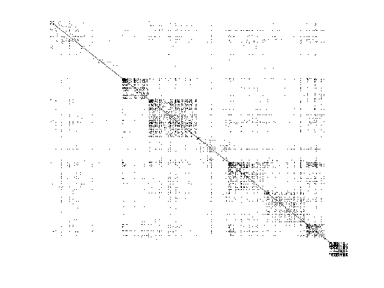
注意：罚参数lamda的设定对逆协方差的稀疏性的影响很大，可以用交叉验证方式得到。

4.2 方法二

graphicalLasso.m

function [Theta, W] = graphicalLasso(S, rho, maxIt, tol)
% http://www.ece.ubc.ca/~xiaohuic/code/glasso/glasso.htm
% Solve the graphical Lasso
% minimize_{Theta > 0} tr(S*Theta) - logdet(Theta) + rho * ||Theta||_1
% Ref: Friedman et al. (2007) Sparse inverse covariance estimation with the
% graphical lasso. Biostatistics.
% Note: This function needs to call an algorithm that solves the Lasso
% problem. Here, we choose to use to the function *lassoShooting* (shooting
% algorithm) for this purpose. However, any Lasso algorithm in the
% penelized form will work.
%
% Input:
% S -- sample covariance matrix
% rho --  regularization parameter
% maxIt -- maximum number of iterations
% tol -- convergence tolerance level
%
% Output:
% Theta -- inverse covariance matrix estimate
% W -- regularized covariance matrix estimate, W = Theta^-1
 
p = size(S,1);
 
if nargin < 4, tol = 1e-6; end
if nargin < 3, maxIt = 1e2; end
 
% Initialization
W = S + rho * eye(p);   % diagonal of W remains unchanged
W_old = W;
i = 0;
 
% Graphical Lasso loop
while i < maxIt,
    i = i+1;
    for j = p:-1:1,
        jminus = setdiff(1:p,j);
        [V D] = eig(W(jminus,jminus));
        d = diag(D);
        X = V * diag(sqrt(d)) * V'; % W_11^(1/2)
        Y = V * diag(1./sqrt(d)) * V' * S(jminus,j);    % W_11^(-1/2) * s_12
        b = lassoShooting(X, Y, rho, maxIt, tol);
        W(jminus,j) = W(jminus,jminus) * b;
        W(j,jminus) = W(jminus,j)';
    end
    % Stop criterion
    if norm(W-W_old,1) < tol, 
        break; 
    end
    W_old = W;
end
if i == maxIt,
    fprintf('%s\n', 'Maximum number of iteration reached, glasso may not converge.');
end
 
Theta = W^-1;
 
% Shooting algorithm for Lasso (unstandardized version)
function b = lassoShooting(X, Y, lambda, maxIt, tol),
 
if nargin < 4, tol = 1e-6; end
if nargin < 3, maxIt = 1e2; end
 
% Initialization
[n,p] = size(X);
if p > n,
    b = zeros(p,1); % From the null model, if p > n
else
    b = X \ Y;  % From the OLS estimate, if p <= n
end
b_old = b;
i = 0;
 
% Precompute X'X and X'Y
XTX = X'*X;
XTY = X'*Y;
 
% Shooting loop
while i < maxIt,
    i = i+1;
    for j = 1:p,
        jminus = setdiff(1:p,j);
        S0 = XTX(j,jminus)*b(jminus) - XTY(j);  % S0 = X(:,j)'*(X(:,jminus)*b(jminus)-Y)
        if S0 > lambda,
            b(j) = (lambda-S0) / norm(X(:,j),2)^2;
        elseif S0 < -lambda,
            b(j) = -(lambda+S0) / norm(X(:,j),2)^2;
        else
            b(j) = 0;
        end
    end
    delta = norm(b-b_old,1);    % Norm change during successive iterations
    if delta < tol, break; end
    b_old = b;
end
if i == maxIt,
    fprintf('%s\n', 'Maximum number of iteration reached, shooting may not converge.');
end

结果

>> A=[5.9436    0.0676    0.5844   -0.0143
    0.0676    0.5347   -0.0797   -0.0115
    0.5844   -0.0797    6.3648   -0.1302
   -0.0143   -0.0115   -0.1302    0.2389
];
>> [Theta, W] = graphicalLasso(A, 1e-4)
 
Theta =
 
    0.1701   -0.0238   -0.0159    0.0003
   -0.0238    1.8792    0.0278    0.1034
   -0.0159    0.0278    0.1607    0.0879
    0.0003    0.1034    0.0879    4.2369
 
 
W =
 
    5.9437    0.0675    0.5843   -0.0142
    0.0675    0.5348   -0.0796   -0.0114
    0.5843   -0.0796    6.3649   -0.1301
   -0.0142   -0.0114   -0.1301    0.2390