

简介
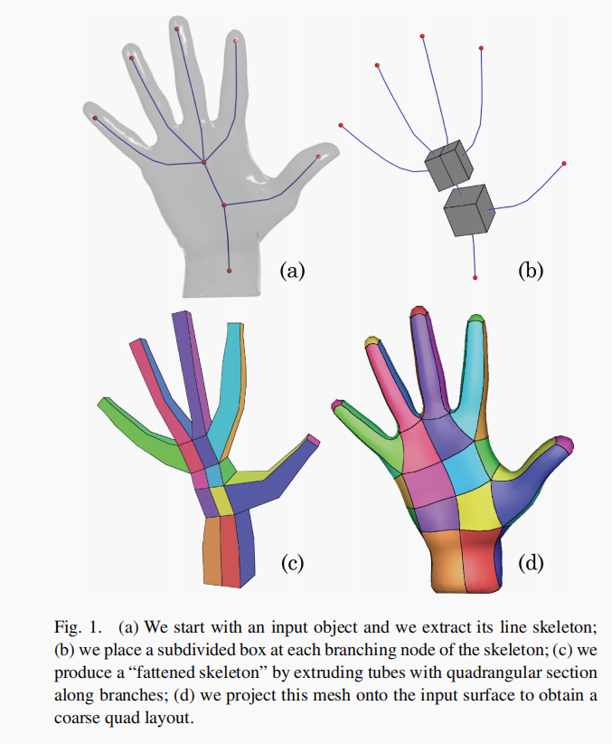
论文简单构述了一个主题,输入三角网格,根据三角网格的骨架信息得到四边形网格
流程步骤
TIPS:
注意红色节点是分支节点和边节点,但是之间其实还是有一部分的折线,逻辑上也是一种节点。这种节点采用的直线的切平面构建的“四边形部分”;
Step 1: 输入三角网格,我们提取他的骨架结构信息
Step 2: 我们放置了一个细分盒子在每一个分支节点处。
Step 3: 我们在沿着管道(分支节点和分支节点,分支节点和边节点)在每个转折处放置一个四边形的面构成一个管道盒子(四边形部分)
Step 4: 我们投影这个网格到输入表面去获得一个粗糙的四边形输出
不足:不能构造精细的网格
作者回顾前人的做法,发现前人没有关于生成粗四边形网格的做法。
奇异点会在分支节点出产生。
基本步骤,生成分支节点六面体,使用整数线性规划方法来调整六面体的站位。
生成六面体。然后参数化将生成的面投影得到原来的面上得到四边形网格。
ILP (整数线性规划问题)
对于一个cubic(立方体)输入的向量\({d_1^i,...d_{k_i}^i}\),我们搜索三个相互垂直的向量\(U_i V_i W_i\)让下面的方程有最下滑的值。
因为绝对值很难进行优化,作者采用了Huang在2014年提出的论文,最小化函数当\(\epsilon \rightarrow 0\)
本来想代码实现这种Ipopt的约束代码,参考了 https://www.coin-or.org/downloading/ ipopt 得在github中才能下载自带的链接可能有错误,可以看看官方给出的帮助pdf。
发现C++实现有一点点复杂。
官方自带例子
// Copyright (C) 2009 International Business Machines.
// All Rights Reserved.
// This code is published under the Eclipse Public License.
//
// $Id: TutorialCpp_main.cpp 1864 2010-12-22 19:21:02Z andreasw $
//
// Author:  Andreas Waechter               IBM    2009-04-02

// This file is part of the Ipopt tutorial.  It is a version with
// mistakes for the C++ implemention of the coding exercise problem
// (in AMPL formulation):
//
// param n := 4;
//
// var x {1..n} <= 0, >= -1.5, := -0.5;
//
// minimize obj:
//   sum{i in 1..n} (x[i]-1)^2;
//
// subject to constr {i in 2..n-1}:
//   (x[i]^2+1.5*x[i]-i/n)*cos(x[i+1]) - x[i-1] = 0;
//
// The constant term "i/n" in the constraint is supposed to be input data
//

#include <cstdio>

#include "IpIpoptApplication.hpp"
#include "TutorialCpp_nlp.hpp"

using namespace Ipopt;

int main(int argv, char* argc[])
{
  // Set the data:

  // Number of variables
  Index N = 5; //100;

  // constant terms in the constraints
  Number* a = new double[N-2];
  for (Index i=0; i<N-2; i++) {
    a[i] = (double(i+2))/(double)N;
  }

  // Create a new instance of your nlp
  //  (use a SmartPtr, not raw)
  SmartPtr<TNLP> mynlp = new TutorialCpp_NLP(N, a);

  // Create a new instance of IpoptApplication
  //  (use a SmartPtr, not raw)
  SmartPtr<IpoptApplication> app = new IpoptApplication();

  // Change some options
  // Note: The following choices are only examples, they might not be
  //       suitable for your optimization problem.
  app->Options()->SetNumericValue("tol", 1e-10);
  app->Options()->SetStringValue("mu_strategy", "adaptive");

  // Intialize the IpoptApplication and process the options
  app->Initialize();

  // Ask Ipopt to solve the problem
  ApplicationReturnStatus status = app->OptimizeTNLP(mynlp);

  if (status == Solve_Succeeded) {
    printf("\n\n*** The problem solved!\n");
  }
  else {
    printf("\n\n*** The problem FAILED!\n");
  }

  // As the SmartPtrs go out of scope, the reference count
  // will be decremented and the objects will automatically
  // be deleted.

  // However, we created the Number array for a here and have to delete it
  delete [] a;

  return (int) status;
}
// Copyright (C) 2009 International Business Machines.
// All Rights Reserved.
// This code is published under the Eclipse Public License.
//
// $Id: TutorialCpp_nlp.hpp 1864 2010-12-22 19:21:02Z andreasw $
//
// Author:  Andreas Waechter               IBM    2009-04-02

// This file is part of the Ipopt tutorial.  It is a version with
// mistakes for the C++ implemention of the coding exercise problem
// (in AMPL formulation):
//
// param n := 4;
//
// var x {1..n} <= 0, >= -1.5, := -0.5;
//
// minimize obj:
//   sum{i in 1..n} (x[i]-1)^2;
//
// subject to constr {i in 2..n-1}:
//   (x[i]^2+1.5*x[i]-i/n)*cos(x[i+1]) - x[i-1] = 0;
//
// The constant term "i/n" in the constraint is supposed to be input data
//

#ifndef __TUTORIALCPP_NLP_HPP__
#define __TUTORIALCPP_NLP_HPP__

#include "IpTNLP.hpp"

using namespace Ipopt;

// This inherits from Ipopt's TNLP
class TutorialCpp_NLP : public TNLP
{
public:
  /** constructor that takes in problem data */
  TutorialCpp_NLP(Index N, const Number* a);

  /** default destructor */
  virtual ~TutorialCpp_NLP();

  /**@name Overloaded from TNLP */
  //@{
  /** Method to return some info about the nlp */
  virtual bool get_nlp_info(Index& n, Index& m, Index& nnz_jac_g,
                            Index& nnz_h_lag, IndexStyleEnum& index_style);

  /** Method to return the bounds for my problem */
  virtual bool get_bounds_info(Index n, Number* x_l, Number* x_u,
                               Index m, Number* g_l, Number* g_u);

  /** Method to return the starting point for the algorithm */
  virtual bool get_starting_point(Index n, bool init_x, Number* x,
                                  bool init_z, Number* z_L, Number* z_U,
                                  Index m, bool init_lambda,
                                  Number* lambda);

  /** Method to return the objective value */
  virtual bool eval_f(Index n, const Number* x, bool new_x, Number& obj_value);

  /** Method to return the gradient of the objective */
  virtual bool eval_grad_f(Index n, const Number* x, bool new_x, Number* grad_f);

  /** Method to return the constraint residuals */
  virtual bool eval_g(Index n, const Number* x, bool new_x, Index m, Number* g);

  /** Method to return:
   *   1) The structure of the jacobian (if "values" is NULL)
   *   2) The values of the jacobian (if "values" is not NULL)
   */
  virtual bool eval_jac_g(Index n, const Number* x, bool new_x,
                          Index m, Index nele_jac, Index* iRow, Index *jCol,
                          Number* values);

  /** Method to return:
   *   1) The structure of the hessian of the lagrangian (if "values" is NULL)
   *   2) The values of the hessian of the lagrangian (if "values" is not NULL)
   */
  virtual bool eval_h(Index n, const Number* x, bool new_x,
                      Number obj_factor, Index m, const Number* lambda,
                      bool new_lambda, Index nele_hess, Index* iRow,
                      Index* jCol, Number* values);

  //@}

  /** @name Solution Methods */
  //@{
  /** This method is called when the algorithm is complete so the TNLP can store/write the solution */
  virtual void finalize_solution(SolverReturn status,
                                 Index n, const Number* x, const Number* z_L, const Number* z_U,
                                 Index m, const Number* g, const Number* lambda,
                                 Number obj_value,
				 const IpoptData* ip_data,
				 IpoptCalculatedQuantities* ip_cq);
  //@}

private:
  /**@name Methods to block default compiler methods.
   * The compiler automatically generates the following three methods.
   *  Since the default compiler implementation is generally not what
   *  you want (for all but the most simple classes), we usually
   *  put the declarations of these methods in the private section
   *  and never implement them. This prevents the compiler from
   *  implementing an incorrect "default" behavior without us
   *  knowing. (See Scott Meyers book, "Effective C++")
   *
   */
  //@{
  TutorialCpp_NLP();
  TutorialCpp_NLP(const TutorialCpp_NLP&);
  TutorialCpp_NLP& operator=(const TutorialCpp_NLP&);
  //@}

  /** @name NLP data */
  //@{
  /** Number of variables */
  Index N_;
  /** Value of constants in constraints */
  Number* a_;
  //@}
};


#endif
// Copyright (C) 2009 International Business Machines.
// All Rights Reserved.
// This code is published under the Eclipse Public License.
//
// $Id: TutorialCpp_nlp.cpp 1864 2010-12-22 19:21:02Z andreasw $
//
// Author:  Andreas Waechter               IBM    2009-04-02

// This file is part of the Ipopt tutorial.  It is a version with
// mistakes for the C++ implemention of the coding exercise problem
// (in AMPL formulation):
//
// param n := 4;
//
// var x {1..n} <= 0, >= -1.5, := -0.5;
//
// minimize obj:
//   sum{i in 1..n} (x[i]-1)^2;
//
// subject to constr {i in 2..n-1}:
//   (x[i]^2+1.5*x[i]-i/n)*cos(x[i+1]) - x[i-1] = 0;
//
// The constant term "i/n" in the constraint is supposed to be input data
//

#include "TutorialCpp_nlp.hpp"

#include <cstdio>

// We use sin and cos
#include <cmath>

using namespace Ipopt;

// constructor
TutorialCpp_NLP::TutorialCpp_NLP(Index N, const Number* a)
  :
  N_(N)
{
  // Copy the values for the constants appearing in the constraints
  a_ = new Number[N_-2];
  for (Index i=0; i<N_-2; i++) {
    a_[i] = a[i];
  }
}

//destructor
TutorialCpp_NLP::~TutorialCpp_NLP()
{
  // make sure we delete everything we allocated
  delete [] a_;
}

// returns the size of the problem
bool TutorialCpp_NLP::get_nlp_info(Index& n, Index& m, Index& nnz_jac_g,
				   Index& nnz_h_lag,
				   IndexStyleEnum& index_style)
{
  // number of variables is given in constructor
  n = N_;

  // we have N_-2 constraints
  m = N_-2;

  // each constraint has three nonzeros
  nnz_jac_g = 3*m;

  // We have the full diagonal, and the first off-diagonal except for
  // the first and last variable
  nnz_h_lag = n + (n-2);

  // use the C style indexing (0-based) for the matrices
  index_style = TNLP::C_STYLE;

  return true;
}

// returns the variable bounds
bool TutorialCpp_NLP::get_bounds_info(Index n, Number* x_l, Number* x_u,
				      Index m, Number* g_l, Number* g_u)
{
  // here, the n and m we gave IPOPT in get_nlp_info are passed back to us.
  // If desired, we could assert to make sure they are what we think they are.
  assert(n == N_);
  assert(m == N_-2);

  // the variables have lower bounds of -1.5
  for (Index i=0; i<n; i++) {
    x_l[i] = -1.5;
  }

  // the variables have upper bounds of 0
  for (Index i=0; i<n; i++) {
    x_u[i] = 0.;
  }

  // all constraints are equality constraints with right hand side zero
  for (Index j=0; j<m; j++) {
    g_l[j] = g_u[j] = 0.;
  }

  return true;
}

// returns the initial point for the problem
bool TutorialCpp_NLP::get_starting_point(Index n, bool init_x, Number* x,
					 bool init_z, Number* z_L, Number* z_U,
					 Index m, bool init_lambda,
					 Number* lambda)
{
  // Here, we assume we only have starting values for x, if you code
  // your own NLP, you can provide starting values for the dual variables
  // if you wish
  assert(init_x == true);
  assert(init_z == false);
  assert(init_lambda == false);

  // initialize to the given starting point
  for (Index i=0; i<n; i++) {
    x[i] = -0.5;
  }

//#define skip_me
#ifdef skip_me
  /* If checking derivatives, if is useful to choose different values */
  for (Index i=0; i<n; i++) {
    x[i] = -0.5+0.1*i/n;
  }
#endif

  return true;
}

// returns the value of the objective function
// sum{i in 1..n} (x[i]-1)^2;
bool TutorialCpp_NLP::eval_f(Index n, const Number* x,
			     bool new_x, Number& obj_value)
{
  assert(n == N_);

  obj_value = 0.;
  for (Index i=0; i<n; i++) {
    obj_value += (x[i]-1.)*(x[i]-1.);
  }

  return true;
}

// return the gradient of the objective function grad_{x} f(x)
bool TutorialCpp_NLP::eval_grad_f(Index n, const Number* x,
				  bool new_x, Number* grad_f)
{
  assert(n == N_);

  for (Index i=1; i<n; i++) {
    grad_f[i] = 2.*(x[i]-1.);
  }

  return true;
}

// return the value of the constraints: g(x)
// (x[j+1]^2+1.5*x[j+1]-a[j])*cos(x[j+2]) - x[j] = 0;
bool TutorialCpp_NLP::eval_g(Index n, const Number* x,
			     bool new_x, Index m, Number* g)
{
  assert(n == N_);
  assert(m == N_-2);

  for (Index j=0; j<m; j++) {
    g[j] = (x[j+1]*x[j+1] + 1.5*x[j+1] -a_[j])*cos(x[j+2]) - x[j];
  }

  return true;
}

// return the structure or values of the jacobian
bool TutorialCpp_NLP::eval_jac_g(Index n, const Number* x, bool new_x,
				 Index m, Index nele_jac, Index* iRow,
				 Index *jCol, Number* values)
{
  if (values == NULL) {
    // return the structure of the jacobian

    Index inz = 0;
    for (Index j=0; j<m; j++) {
      iRow[inz] = j;
      jCol[inz] = j;
      inz++;
      iRow[inz] = j;
      jCol[inz] = j+1;
      inz++;
      iRow[inz] = j;
      jCol[inz] = j+1;
      inz++;
    }
    // sanity check
    assert(inz==nele_jac);
  }
  else {
    // return the values of the jacobian of the constraints

    Index inz = 0;
    for (Index j=0; j<m; j++) {
      values[inz] = 1.;
      inz++;
      values[inz] = (2.*x[j+1]+1.5)*cos(x[j+2]);
      inz++;
      values[inz] = -(x[j+1]*x[j+1] + 1.5*x[j+1] -a_[j])*sin(x[j+2]);
      inz++;
    }
    // sanity check
    assert(inz==nele_jac);
  }

  return true;
}

//return the structure or values of the hessian
bool TutorialCpp_NLP::eval_h(Index n, const Number* x, bool new_x,
			     Number obj_factor, Index m, const Number* lambda,
			     bool new_lambda, Index nele_hess, Index* iRow,
			     Index* jCol, Number* values)
{
  if (values == NULL) {

    Index inz = 0;

    // First variable has only a diagonal entry
    iRow[inz] = 0;
    jCol[inz] = 0;
    inz++;

    // Next ones have first off-diagonal and diagonal
    for (Index i=1; i<n-1; i++) {
      iRow[inz] = i;
      jCol[inz] = i;
      inz++;
      iRow[inz] = i;
      jCol[inz] = i+1;
      inz++;
    }

    // Last variable has only a diagonal entry
    iRow[inz] = n-2;
    jCol[inz] = n-2;
    inz++;

    assert(inz == nele_hess);
  }
  else {
    // return the values. This is a symmetric matrix, fill the upper right
    // triangle only

    Index inz = 0;

    // Diagonal entry for first variable
    values[inz] = obj_factor*2.;
    inz++;

    for (Index i=1; i<n-1; i++) {
      values[inz] = obj_factor*2. + lambda[i-1]*2.*cos(x[i+1]);
      if (i>1) {
	values[inz] -= lambda[i-2]*(x[i]*x[i] + 1.5*x[i-1] -a_[i-2])*cos(x[i]);
      }
      inz++;
      values[inz] = -lambda[i-1]*(2.*x[i]+1.5)*sin(x[i+1]);
      inz++;
    }

    values[inz] = obj_factor*2.;
    values[inz] -= lambda[n-3]*(x[n-1]*x[n-1] + 1.5*x[n-2] -a_[n-3])*cos(x[n-1]);
    inz++;

    assert(inz == nele_hess);
  }

  return true;
}

void TutorialCpp_NLP::finalize_solution(SolverReturn status,
					Index n, const Number* x,
					const Number* z_L, const Number* z_U,
					Index m, const Number* g,
					const Number* lambda,
					Number obj_value,
					const IpoptData* ip_data,
					IpoptCalculatedQuantities* ip_cq)
{
  // here is where we would store the solution to variables, or write
  // to a file, etc so we could use the solution.

  printf("\nWriting solution file solution.txt\n");
  FILE* fp = fopen("solution.txt", "w");

  // For this example, we write the solution to the console
  fprintf(fp, "\n\nSolution of the primal variables, x\n");
  for (Index i=0; i<n; i++) {
    fprintf(fp, "x[%d] = %e\n", i, x[i]);
  }

  fprintf(fp, "\n\nSolution of the bound multipliers, z_L and z_U\n");
  for (Index i=0; i<n; i++) {
    fprintf(fp, "z_L[%d] = %e\n", i, z_L[i]);
  }
  for (Index i=0; i<n; i++) {
    fprintf(fp, "z_U[%d] = %e\n", i, z_U[i]);
  }

  fprintf(fp, "\n\nObjective value\n");
  fprintf(fp, "f(x*) = %e\n", obj_value);
  fclose(fp);
}
中间我看了一下代码用到了求导相关代码的编写。虽然速度很快运行结束。
JN的放置规则
JN是一个四边形的面,他的垂直部分的管道几乎和骨架平行。他垂直于两条入射弧度的平均方向。
BN-EN
因为EN是端点,随意放置规则比较简单,直接沿着Bn的面传播即可
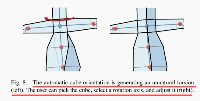
BN-BN。
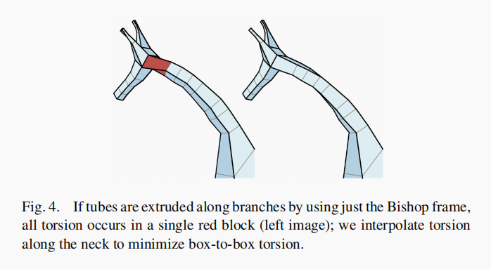
如图所示,红色的四边形是直接扭转,但是右边的图形看起来好很多因为加入了面对面的插值扭转。
因为是对应着两个面所以,中间所插入的四边形JN需要设定一定插值扭转
分裂传递
对于每个BN和EN采用防止cube 的方案,总所周知切分一个正方体有对上面有两种切法,横着切竖着切,对于侧面有一种切法,横着切(侧面的竖着切由上面实现)。
对于中间的JN有两种切法横着切和竖着切。
3n * 2m // n表示分支节点和终端节点的个数,m表示管道节点的个数,总共的未知变量就是此公式
简单来说构建一个整数线性规划问题。但是具体我不是特别清楚如何构建。
作者讲述了对于一个BN,那么将每一个面构造两个主方向U和V。然后管道和BN相遇之后我们需要将BN细分就是保持拓扑一致。
感觉有点麻烦。可以用编程简单实现而不用构造一个ILP方程。虽然编程也不容易实现。
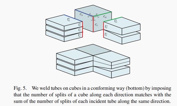
观图易知对于CUBE有三个变量分别是UVW方向上的线段切分数量和切分点而管道只有两个变量UV。
具体如何构建方程我不是特别清楚,如果谁知道麻烦在下面留言
障碍
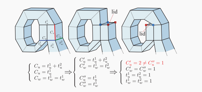
可以从图中看出对于第一个图,采用编程方案可能导致循环分裂,作者通过人为或者编程(没细看)破解了这种循环。
粗四边形网格和映射
\(\mathcal{M}\) 表示初始的三角网格
\(\mathcal{Q}\) 表示粗四边形网格
节点boxes(盒子)的大小是中心点到M内切球半径的大小。
初始化投影
将Q的每个顶点沿着Q的面法向投影到M,选择M中离Q的投影点最近的点作为映射
细分
将Q进行CC细分,然后每个点按照之前的方式投影到M上。
逆投影
M中的点也投影到Q中
通过参数化的手段优化顶点的位置,具体没有看的特别懂,如果要懂可能要看相关的作者所引用的论文了。
提出了什么共形能量,但是没有看懂。
Resizing
没看懂
用户交互
可以调整BN的角度XYZ方向
增加分支节点
Retouching Parameterization.
没看懂
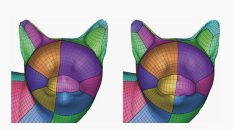
似乎好像猫的鼻子那里出现了对称的情况。
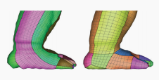
结果展示
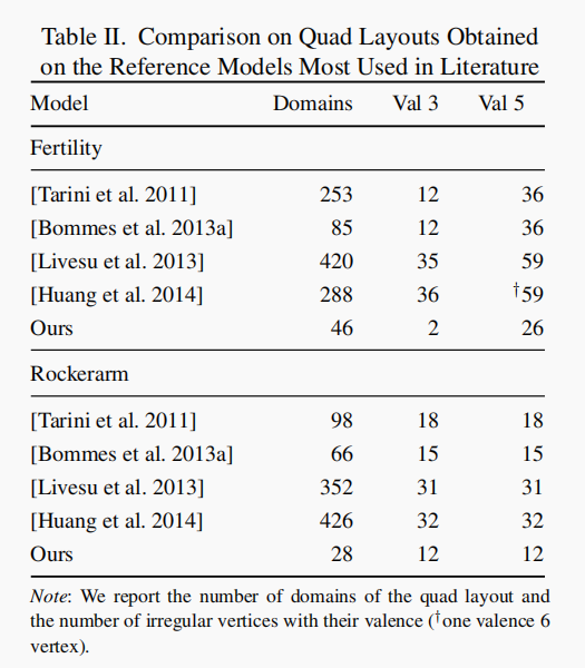
作者的方法可以生成更少的主面片区域
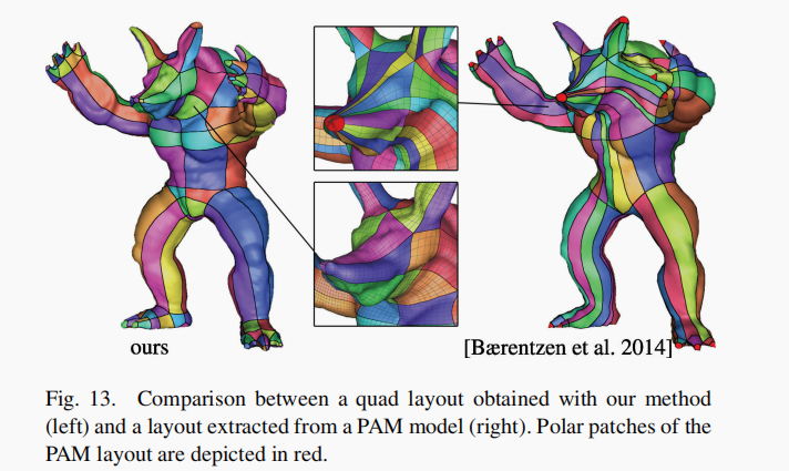
在鼻尖的展示更好
产生更小的相对标准偏差relative standard deviation (RSD)
缺点
所有不能用骨架很好的描述的模型,都不能够生成,比如杯子的空腔。
未来的工作
可以通过调整骨架节点来实现对模型的调整。
可以生成六面体网格。
为交叉参数化提供了基础,这可以用于动画的目的。
当前生成的骨架,但是并没有语义化骨架信息,比如给出一个大象的大腿。