一、boston房价预测
1. 读取数据集
2. 训练集与测试集划分
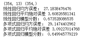
3. 线性回归模型:建立13个变量与房价之间的预测模型,并检测模型好坏。
4. 多项式回归模型:建立13个变量与房价之间的预测模型,并检测模型好坏。
from sklearn.datasets import load_boston  #导入Boston房价数据集
boston = load_boston()   #读取数据集
# boston.keys()    #查看key值
x = boston.data
y = boston.target

#训练集与测试集划分
from sklearn.cross_validation import train_test_split
x_train,x_test,y_train,y_test = train_test_split(x,y,test_size=0.3,random_state=0)
#其中 test_size是样本占比,如果是整数的话就是样本的数量;
#random_state是随机数的种子,不同的种子会造成不同的随机采样结果,相同的种子采样结果相同。
print(x_train.shape,y_train.shape)

#建立一元线性回归模型
from sklearn.linear_model import LinearRegression
lr = LinearRegression()
lr.fit(x_train,y_train)
lr.coef_    #系数
lr.intercept_   #截距


#检测模型好坏
from sklearn.metrics import regression
y_pred = lr.predict(x_test)   #预测
n = regression.mean_squared_error(y_test,y_pred) #预测模型均方误差
print("线性回归均方误差:",n)
a = regression.mean_absolute_error(y_test,y_pred)
print("线性回归平均绝对误差",a)
s = lr.score(x_test,y_test)  #模型分数
print("线性回归模型分数:",s)


#多元多项式回归模型
from sklearn.preprocessing import PolynomialFeatures
poly= PolynomialFeatures(degree=2)
x_poly_train= poly.fit_transform(x_train) #多项式化
x_poly_test  = poly.transform(x_test)

#建立模型
lr2 = LinearRegression()
lr2.fit(x_poly_train,y_train)

#预测
y_pred2 = lr2.predict(x_poly_test)

#检测模型好坏,计算模型的预测指标
n2 = regression.mean_squared_error(y_test,y_pred2)
print("多项式回归均方误差:",n2)
a2 = regression.mean_absolute_error(y_test,y_pred2)
print("多项式回归平均绝对误差",a2)
s2 = lr2.score(x_poly_test,y_test)
print("多项式回归模型分数:",s2)
# 用一元线性回归拟合观察效果
lr2 = LinearRegression()
lr2.fit(x,y_train)
# 建立多项式模型
from sklearn.preprocessing import PolynomialFeatures
# 多项式化x
x = x_train[:,12].reshape(-1,1)
poly= PolynomialFeatures(degree=2)
x_poly = poly.fit_transform(x)

# 用多项式后的x建立多项式回归模型
lrp = LinearRegression()
lrp.fit(x_poly,y_train)

# 预测
x_poly2 = poly.transform(x_test[:, 12].reshape(-1,1))
y_ploy_predict = lrp.predict(x_poly2)

# 图形化,将元数据,一元拟合,多元拟合进行绘图观察
plt.scatter(x_test[:,12], y_test)
plt.plot(x, lr2.coef_* x + lr2.intercept_, 'g')
plt.scatter(x_test[:,12], y_ploy_predict, c='r')
plt.show()

5、比较线性模型与非线性模型的性能,并说明原因。
如上图可知,非线性模型的性能比较好,因为非线性模型(即多项式回归模型)的曲线比线性模型直线更能契合人口密度与房屋样本的分布状况,而且从上述分析可知多项式回归的误差跟线性回归误差相比较小。
二、中文文本分类
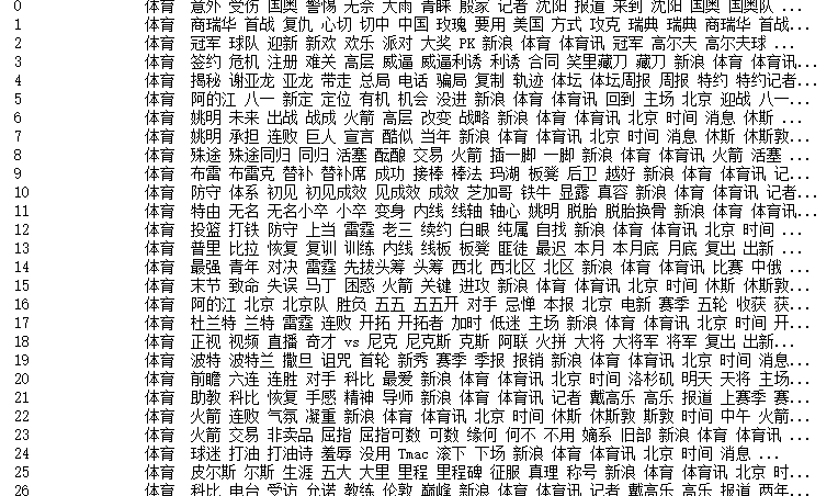
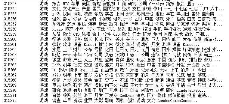
import os
import numpy as np
import sys
from datetime import datetime
import gc
path = 'E:\\大三\\数据挖掘\\qimo\\0369'

# 导入结巴库,并将需要用到的词库加进字典
import jieba
# 导入停用词:
with open(r'E:\大三\数据挖掘\qimo\stopsCN.txt', encoding='utf-8') as f:
    stopwords = f.read().split('\n')

#预处理数据,先定义一个函数,然后封装
def processing(tokens):
    # 去掉非字母汉字的字符,isalpha判断字符ch是否为英文字母,若为英文字母,返回非0(小写字母为2,大写字母为1)。若不是字母,返回0。
    tokens = "".join([char for char in tokens if char.isalpha()])
    # 结巴分词,砍掉大于等于2个以上的词,(即将一句话拆分为各个词语)
    tokens = [token for token in jieba.cut(tokens,cut_all=True) if len(token) >=2]
    # 去掉停用词
    tokens = " ".join([token for token in tokens if token not in stopwords])
    return tokens

tokenList = []
targetList = []
# 用os.walk获取需要的变量,并拼接文件路径再打开每一个文件
for root,dirs,files in os.walk(path):
    for f in files:
#     print(root)    #当前目录路径
#     print(dirs)    #当前路径下所有子目录
#     print(files)   #当前路径下所有非目录子文件
        filePath = os.path.join(root,f)
        with open(filePath, encoding='utf-8') as f:
            content = f.read()     #存放读取的数据
            # 获取新闻类别标签,并处理该新闻
        target = filePath.split('\\')[-2]
        targetList.append(target)            #获取的新闻文本的类别,追加到targetList里
        tokenList.append(processing(content))   #获取的各新闻文本里的详细内容,预处理后追加到tokenList

import pandas
datas = pandas.DataFrame({
    'targetList': targetList,
    'tokenList':  tokenList
})
print(datas)
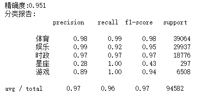
#划分训练集测试集并建立特征向量,为建立模型做准备
#划分训练集、测试集
from sklearn.model_selection import train_test_split
x_train,x_test,y_train,y_test= train_test_split(tokenList,targetList,test_size=0.3,stratify=targetList)

#转化为特征向量。
from sklearn.feature_extraction.text import TfidfVectorizer
vec = TfidfVectorizer()
x_train = vec.fit_transform(x_train)
x_test = vec.transform(x_test)

#建立模型,因为样本特征的a分布大部分是多元离散值,所以用多项式朴素贝叶斯
from sklearn.naive_bayes import GaussianNB,MultinomialNB
mnb = MultinomialNB()
module = mnb.fit(x_train,y_train)

#进行预测
y_pred = module.predict(x_test)

#输出模型精确度
from sklearn.model_selection import cross_val_score
scores = cross_val_score(mnb,x_test,y_test,cv=5)
print("精确度:%.3f"%scores.mean())
#输出模型评估报告,
from sklearn.metrics import classification_report
print("分类报告:\n",classification_report(y_pred,y_test))
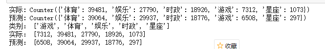
#将预测结果和实际结果进行对比
import collections
import matplotlib.pyplot as plt
from pylab import mpl

# mpl.rcParams['font.sans-serif'] = ['FangSong']  #指定默认仿宋字体
# mpl.reParams['axes.unicode_minus'] = False     #解决保存图像是负号‘-’显示为方块的问题、

mpl.rcParams['font.sans-serif'] = ['FangSong'] # 指定默认字体
mpl.rcParams['axes.unicode_minus'] = False # 解决保存图像是负号'-'显示为方块的问题

#统计测试集和预测集的各类新闻文本个数
testCount = collections.Counter(y_test)
predCount = collections.Counter(y_pred)
print('实际:',testCount)
print('预测:',predCount)

#建立标签列表,实际结果列表和预测结果列表
nameList = list(testCount.keys())
testList = list(testCount.values())
predList = list(predCount.values())
x = list(range(len(nameList)))
print("类别:",nameList)
print("实际:",testList)
print("预测:",predList)