

衡量回归算法的标准
import numpy as np
import matplotlib.pyplot as plt
from sklearn import datasets
波士顿房产数据
boston_market = datasets.load_boston()
print(boston_market.DESCR)
.. _boston_dataset:

Boston house prices dataset
---------------------------

**Data Set Characteristics:**

    :Number of Instances: 506

    :Number of Attributes: 13 numeric/categorical predictive. Median Value (attribute 14) is usually the target.

    :Attribute Information (in order):
        - CRIM     per capita crime rate by town
        - ZN       proportion of residential land zoned for lots over 25,000 sq.ft.
        - INDUS    proportion of non-retail business acres per town
        - CHAS     Charles River dummy variable (= 1 if tract bounds river; 0 otherwise)
        - NOX      nitric oxides concentration (parts per 10 million)
        - RM       average number of rooms per dwelling
        - AGE      proportion of owner-occupied units built prior to 1940
        - DIS      weighted distances to five Boston employment centres
        - RAD      index of accessibility to radial highways
        - TAX      full-value property-tax rate per $10,000
        - PTRATIO  pupil-teacher ratio by town
        - B        1000(Bk - 0.63)^2 where Bk is the proportion of blacks by town
        - LSTAT    % lower status of the population
        - MEDV     Median value of owner-occupied homes in $1000's

    :Missing Attribute Values: None

    :Creator: Harrison, D. and Rubinfeld, D.L.

This is a copy of UCI ML housing dataset.
https://archive.ics.uci.edu/ml/machine-learning-databases/housing/

This dataset was taken from the StatLib library which is maintained at Carnegie Mellon University.

The Boston house-price data of Harrison, D. and Rubinfeld, D.L. 'Hedonic
prices and the demand for clean air', J. Environ. Economics & Management,
vol.5, 81-102, 1978.   Used in Belsley, Kuh & Welsch, 'Regression diagnostics
...', Wiley, 1980.   N.B. Various transformations are used in the table on
pages 244-261 of the latter.

The Boston house-price data has been used in many machine learning papers that address regression
problems.

.. topic:: References

   - Belsley, Kuh & Welsch, 'Regression diagnostics: Identifying Influential Data and Sources of Collinearity', Wiley, 1980. 244-261.
   - Quinlan,R. (1993). Combining Instance-Based and Model-Based Learning. In Proceedings on the Tenth International Conference of Machine Learning, 236-243, University of Massachusetts, Amherst. Morgan Kaufmann.
print(boston_market.feature_names)
['CRIM' 'ZN' 'INDUS' 'CHAS' 'NOX' 'RM' 'AGE' 'DIS' 'RAD' 'TAX' 'PTRATIO'
'B' 'LSTAT']
x = boston_market.data[:, 5]
#只取房间数量这个特征
y = boston_market.target
print(x.shape)
print(y.shape)
(506,)
(506,)
#绘制图像
plt.scatter(x, y)
plt.show()
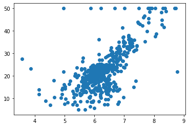
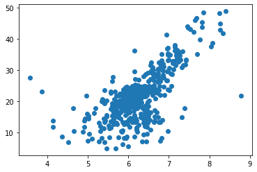
#我们发现有一些点都是50,这是由于统计时候造成的,所以将这些点剔除掉
x = x[y < 50]
y = y[y < 50]
plt.scatter(x, y)
plt.show()
使用我们自己封装的简单线性回归法
使用pycharm在同级目录下新建工程play_ML
新建py脚本命名为model_selection
写入以下代码
import numpy as np


def train_test_split(X, y, train_ratio = 0.8, seed = None):
    '''将数据X和y按照train_ratio的比例划分为X_train, y_train, X_test, y_test'''
    assert X.shape[0] == y.shape[0], \
    "the size of X must be equal to the size of y"
    assert 0.0 <= train_ratio <= 1.0, \
    "train_ratio must be valid"

    if seed:
        np.random.seed(seed)

    shuffled_indexes = np.random.permutation(len(X))

    train_size = int(len(X) * train_ratio)
    train_indexes = shuffled_indexes[:train_size]
    test_indexes = shuffled_indexes[train_size:]

    X_train = X[train_indexes]
    y_train = y[train_indexes]

    X_test = X[test_indexes]
    y_test = y[test_indexes]

    return X_train, X_test, y_train, y_test
导入自定义的类
from play_ML.model_selection import train_test_split

x_train, x_test, y_train, y_test = train_test_split(x, y, seed = 666)
print(x_train.shape)
print(x_test.shape)
(392,)
(98,)
from play_ML.SimpleLinearRegression import SimpleLinearRegression2
reg = SimpleLinearRegression2()
reg.fit(x_train, y_train)
SimpleLinearRegression2()
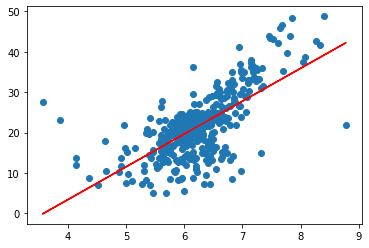
print(reg.a_)
print(reg.b_)
8.123193848801828
-29.07267361874801
#绘制图像
plt.scatter(x_train, y_train)
plt.plot(x_train, reg.predict(x_train), color = "red")
plt.show()
均方误差MSE
y_predict = reg.predict(x_test)
mse_test = np.sum((y_predict - y_test) ** 2) / len(y_test)
mse_test
#单位是(万元)**2
28.418315342489713
均方根误差RMSE
from math import sqrt
rmse_test = sqrt(mse_test)
rmse_test
#单位 万元
5.330883167214389
平均绝对误差MAE
mae_test = np.sum(np.absolute(y_predict - y_test)) / len(y_test)
mae_test
#单位 万元
3.8540656979860923
在play_ML项目中新建py脚本,命名为metrics
写入以下评价指标代码
# 对准确率的计算也进行封装
import numpy as np
from math import sqrt


def accuracy_score(y_true, y_predict):
    """计算y_true和y_predict之间的准确率"""
    assert y_true.shape[0] == y_predict.shape[0], \
        "the size of y_true must be equal to the size of y_predict"

    return np.sum(y_true == y_predict) / len(y_true)


def mean_squared_error(y_true, y_predict):
    assert y_true.shape[0] == y_predict.shape[0], \
        "the size of y_true must be equal to the size of y_predict"

    return np.sum((y_true - y_predict) ** 2) / len(y_true)


def root_mean_squared_error(y_true, y_predict):
    assert y_true.shape[0] == y_predict.shape[0], \
        "the size of y_true must be equal to the size of y_predict"

    return sqrt(mean_squared_error(y_true, y_predict))


def mean_absolute_error(y_true, y_predict):
    assert y_true.shape[0] == y_predict.shape[0], \
        "the size of y_true must be equal to the size of y_predict"

    return np.sum(np.absolute(y_true - y_predict)) / len(y_true)


def r2_score(y_true, y_predict):
    """计算y_true和y_predict之间的R Square"""

    return 1 - mean_squared_error(y_true, y_predict) / np.var(y_true)
导入我们自己的评价指标
from play_ML.metrics import mean_squared_error
from play_ML.metrics import root_mean_squared_error
from play_ML.metrics import mean_absolute_error
mean_squared_error(y_test, y_predict)
28.418315342489713
root_mean_squared_error(y_test, y_predict)
5.330883167214389
mean_absolute_error(y_test, y_predict)
3.8540656979860923
scikit-learn中的MSE和MAE
from sklearn.metrics import mean_squared_error
from sklearn.metrics import mean_absolute_error
mean_squared_error(y_test, y_predict)
28.418315342489713
mean_absolute_error(y_test, y_predict)
3.8540656979860923
R Square
1 - mean_squared_error(y_test, y_predict) / np.var(y_test)
0.5230262449827334
#使用我们自己封装的R Square
from play_ML.metrics import r2_score

r2_score(y_test, y_predict)
0.5230262449827334
scikit-learn 中的R Square
from sklearn.metrics import r2_score

r2_score(y_test, y_predict)
0.5230262449827334
将R Square作为简单线性回归的评价指标
reg.score(x_test, y_test)
0.5230262449827334

 浙公网安备 33010602011771号