CCS - Error Rate Performance of the Detectors

 

Simulation of MIMO Systems

Perform a Monte Carlo simulation to assess the error rate performance of an
(Ny,NR) MIMO system in a Rayleigh fading AWGN channel.

 

Matlab Coding

% MATLAB script for the 2T2R MIMO system

Nt = 2;                                 % No. of transmit antennas
Nr = 2;                                 % No. of receive antennas
S = [1 1 -1 -1; 1 -1 1 -1];             % Reference codebook
Eb = 1;                                 % Energy per bit
EbNo_dB = 0:5:30;                       % Average SNR per bit
No = Eb*10.^(-1*EbNo_dB/10);            % Noise variance
BER_ML = zeros(1,length(EbNo_dB));      % Bit-Error-Rate Initialization
BER_MMSE = zeros(1,length(EbNo_dB));    % Bit-Error-Rate Initialization
BER_ICD = zeros(1,length(EbNo_dB));     % Bit-Error-Rate Initialization

% Maximum Likelihood Detector:
% echo off;
for i = 1:length(EbNo_dB)
    no_errors = 0;
    no_bits = 0;
    while no_errors <= 100
        mu = zeros(1,4);
        s = 2*randi([0 1],Nt,1) - 1;
        no_bits = no_bits + length(s);
        H = (randn(Nr,Nt) + 1i*randn(Nr,Nt))/sqrt(2*Nr);
        noise = sqrt(No(i)/2)*(randn(Nr,1) + 1i*randn(Nr,1));
        y = H*s + noise;
        for j = 1:4
            mu(j) = sum(abs(y - H*S(:,j)).^2);  % Euclidean distance metric
        end
        [Min idx] = min(mu);
        s_h = S(:,idx);
        no_errors = no_errors + nnz(s_h-s);
    end
    BER_ML(i) = no_errors/no_bits;
end


% echo on;
% Minimum Mean-Sqaure-Error (MMSE) Detector:
echo off;
for i = 1:length(EbNo_dB)
    no_errors = 0;
    no_bits = 0;
    while no_errors <= 100
        s = 2*randi([0 1],Nt,1) - 1;
        no_bits = no_bits + length(s);
        H = (randn(Nr,Nt) + 1i*randn(Nr,Nt))/sqrt(2*Nr);
        noise = sqrt(No(i)/2)*(randn(Nr,1) + 1i*randn(Nr,1));
        y = H*s + noise;
        w1 = (H*H' + No(i)*eye(Nr))^(-1) * H(:,1); % Optimum weight vector 1
        w2 = (H*H' + No(i)*eye(Nr))^(-1) * H(:,2); % Optimum weight vector 2
        W = [w1 w2];
        s_h = W'*y;
        for j = 1:Nt
            if s_h(j) >= 0
                s_h(j) = 1;
            else
                s_h(j) = -1;
            end
        end
        no_errors = no_errors + nnz(s_h-s);
    end
    BER_MMSE(i) = no_errors/no_bits;
end

%echo on;

% Inverse Channel Detector:
% echo off;
for i = 1:length(EbNo_dB)
    no_errors = 0;
    no_bits = 0;
    while no_errors <= 100
        s = 2*randi([0 1],Nt,1) - 1;
        no_bits = no_bits + length(s);
        H = (randn(Nr,Nt) + 1i*randn(Nr,Nt))/sqrt(2*Nr);
        noise = sqrt(No(i)/2)*(randn(Nr,1) + 1i*randn(Nr,1));
        y = H*s + noise;
        s_h = H\y;
        for j = 1:Nt
            if s_h(j) >= 0
                s_h(j) = 1;
            else
                s_h(j) = -1;
            end
        end
        no_errors = no_errors + nnz(s_h-s);
    end
    BER_ICD(i) = no_errors/no_bits;
end
% echo on;

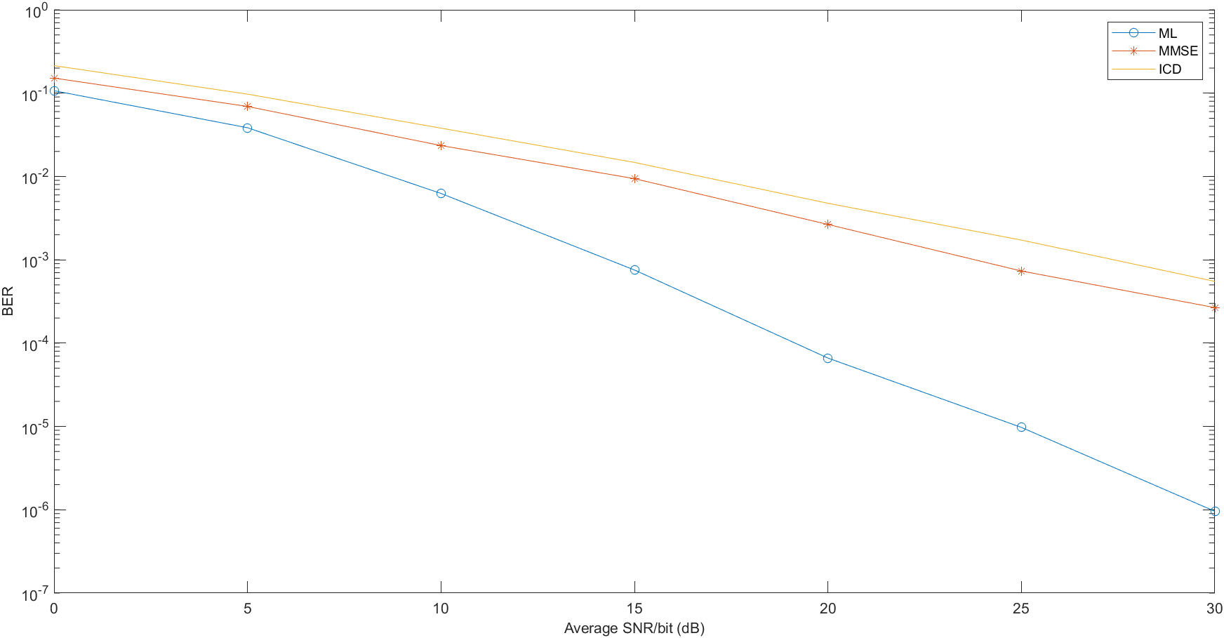
% Plot the results:
semilogy(EbNo_dB,BER_ML,'-o',EbNo_dB,BER_MMSE,'-*',EbNo_dB,BER_ICD)
xlabel('Average SNR/bit (dB)','fontsize',10)
ylabel('BER','fontsize',10)
legend('ML','MMSE','ICD')


Simulation Results,

 

 

 

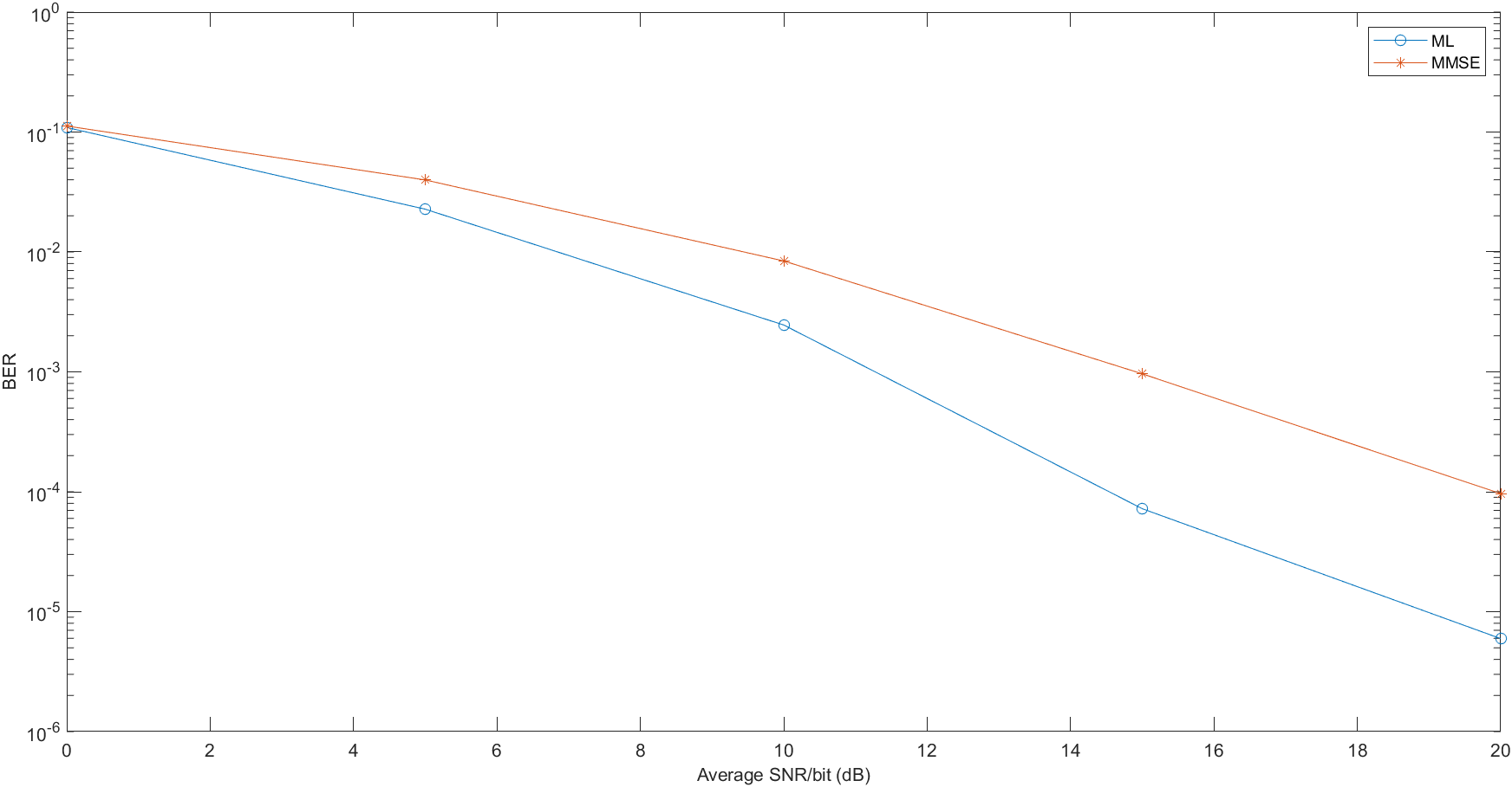
% MATLAB script for 2T3R MIMO system

Nt = 2;                                 % No. of transmit antennas
Nr = 3;                                 % No. of receive antennas
S = [1 1 -1 -1; 1 -1 1 -1];             % Reference codebook
Eb = 1;                                 % Energy per bit
EbNo_dB = 0:5:30;                       % Average SNR per bit
No = Eb*10.^(-1*EbNo_dB/10);            % Noise variance
BER_ML = zeros(1,length(EbNo_dB));      % Bit-Error-Rate Initialization
BER_MMSE = zeros(1,length(EbNo_dB));    % Bit-Error-Rate Initialization
12 
% Maximum Likelihood Detector:
echo off;
for i = 1:length(EbNo_dB)
    no_errors = 0;
    no_bits = 0;
    while no_errors <= 100
        mu = zeros(1,4);
        s = 2*randi([0 1],Nt,1) - 1;
        no_bits = no_bits + length(s);
        H = (randn(Nr,Nt) + 1i*randn(Nr,Nt))/sqrt(2*Nr);
        noise = sqrt(No(i)/2)*(randn(Nr,1) + 1i*randn(Nr,1));
        y = H*s + noise;
        for j = 1:4
            mu(j) = sum(abs(y - H*S(:,j)).^2);  % Euclidean distance metric
        end
        [Min idx] = min(mu);
        s_h = S(:,idx);
        no_errors = no_errors + nnz(s_h-s);
    end
    BER_ML(i) = no_errors/no_bits;
end
echo on;

% Minimum Mean-Sqaure-Error (MMSE) Detector:
echo off;
for i = 1:length(EbNo_dB)
    no_errors = 0;
    no_bits = 0;
    while no_errors <= 100
        s = 2*randi([0 1],Nt,1) - 1;
        no_bits = no_bits + length(s);
        H = (randn(Nr,Nt) + 1i*randn(Nr,Nt))/sqrt(2*Nr);
        noise = sqrt(No(i)/2)*(randn(Nr,1) + 1i*randn(Nr,1));
        y = H*s + noise;
        w1 = (H*H' + No(i)*eye(Nr))^(-1) * H(:,1); % Optimum weight vector 1
        w2 = (H*H' + No(i)*eye(Nr))^(-1) * H(:,2); % Optimum weight vector 2
        W = [w1 w2];
        s_h = W'*y;
        for j = 1:Nt
            if s_h(j) >= 0
                s_h(j) = 1;
            else
                s_h(j) = -1;
            end
        end
        no_errors = no_errors + nnz(s_h-s);
    end
    BER_MMSE(i) = no_errors/no_bits;
end
echo on;

% Plot the results:
semilogy(EbNo_dB,BER_ML,'-o',EbNo_dB,BER_MMSE,'-*')
xlabel('Average SNR/bit (dB)','fontsize',10)
ylabel('BER','fontsize',10)
legend('ML','MMSE')

Simulation Result

 

 

 

Conclusion

It is can be seen from the simulation results that the MLD exploits
the full diversity of order NR available in the received signal and, thus, its performance
is comparable to that of a maximal ratio combiner (MRC) of the NR received signals,
without the presence of interchannel interference; that is, (Ny, NR) = (1, NR). The two
linear detectors, the MMSE detector and the ICD, achieve an error rate that decreases
inversely as the SNR raised to the (NR - 1) power for Ny = 2 transmitting antennas.
Thus, when NR = 2, the two linear detectors achieve no diversity, and when NR = 3,
the linear detectors achieve dual diversity. We also note that the MMSE detector outperforms
the ICD, although both achieve the same order of diversity. In general, with
spatial multiplexing (Ny antennas transmitting independent data streams), the MLD
detector achieves a diversity of order NR and the linear detectors achieve a diversity
of order NR - Ny+ 1, for any NR >= Ny. In effect, with Ny antennas transmitting
independent data streams and NR receiving antennas, a linear detector has NR degrees
of freedom. In detecting any one data stream, in the presence of Ny - 1 interfering
signals from the other transmitting antennas, the linear detectors utilize Ny -1 degrees
of freedom to cancel the Ny - 1 interfering signals. Therefore, the effective order of
diversity for the linear detectors is NR - (Ny -1) = NR - Ny+ 1.

 

It is interesting to compare the computational complexity of the three detectors.
We note that the complexity of the MLD grows exponentially as Af Nr, where M is the
number of points (symbols) in the signal constellation, whereas the linear detectors
have a complexity that grows linearly with Ny and NR. Therefore, the computational
complexity of the MLD is significantly larger than that of the linear detectors when
Ny and M are large. However, for a small number of transmit antennas and small
number of signal constellation symbols (i.e., Ny <= 4 and M = 4), the computational
complexity of MLD is rather reasonable.

 

 

Reference,

　　1. <<Contemporary Communication System using MATLAB>> - John G. Proakis