RPN 图文详解 Faster-RCNN 原文对照

Faster-RCNN and RPN

Contribution

• RPN
  • predefined bboxes(anchors) with different scales

The rest is inherited from Fast RCNN

RPN

learns the proposals from feature maps

🔍 see also RPN

Pipeline

• given raw image \(\mathbb{R}^{H_{0}\times W_{0}}\), feed it to a backbone

the images will be down scaled to \(C_{\text{backbone}}\) tiled feature maps \(\mathbf{f} \in \mathbb{R}^{C_{\text{backbone}} \times H\times W }\)

\[H = \frac{H_{0}}{\mathcal{R}} \]

e.g. for vgg16, the image is reduced by \(\mathcal{R} = 16\) times by the end of the backbone

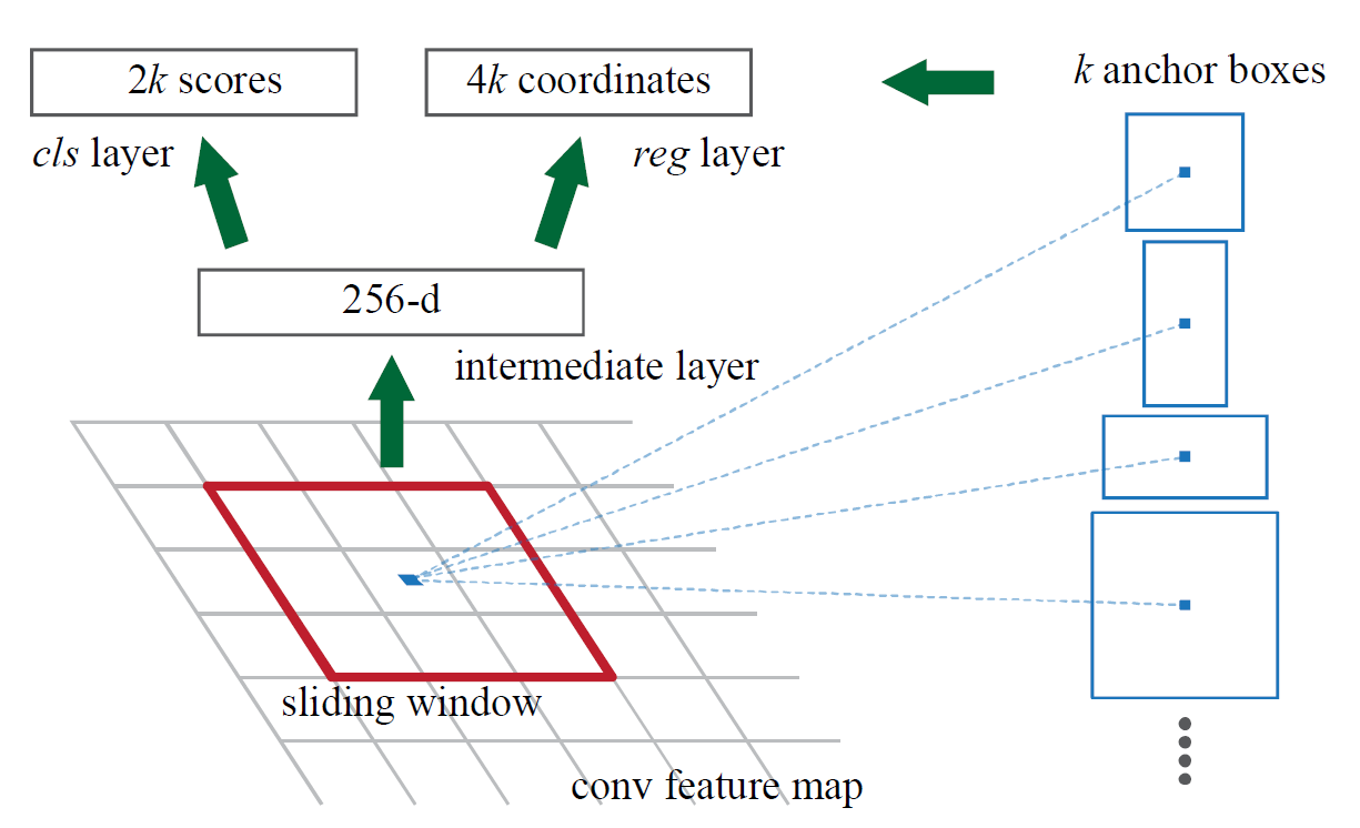
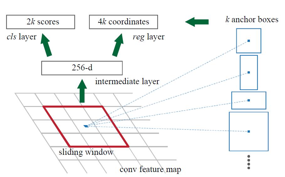
• for each point \(p = (x,y)\) in \(\mathbf{f}\)

First, generate \(k\) anchors

🔍 see below, what are anchors

Then apply a small convnet of size \(n\times n\) centered at \((x,y)\) on the feature map

❗ About how to adjust the predifined anchor boxes

1. this convnet of size \(n\times n\) is compared to sliding window in the paper.
2. this convnet is composed of \(D\) filters, and each filter is of size \(n\times n\)

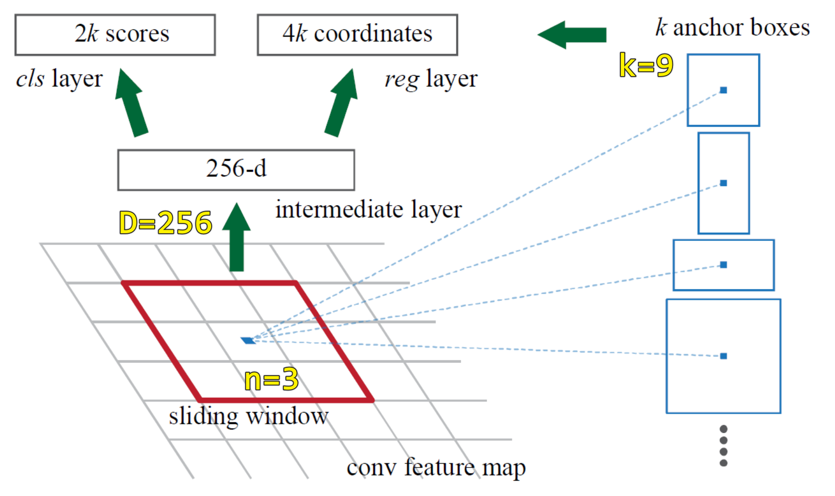
at each point \(p\), \(D=256\) filters will produce \(256\) numbers as a local linear composion(i.e. what CNN does) of a neighbor \(n\times n\).

So, given tiled feature maps \(\mathbf{f} \in \mathbb{R}^{H\times W}\), we will get \(\mathbf{f}_{rpn} \in \mathbb{R}^{256\times H \times W}\)

• apply 1x1 conv to refine anchors

from \(\mathbf{f}_{rpn} \in \mathbb{R}^{256\times H \times W}\) to

1. \(\mathcal{S}_{\text{cls}}\in \mathbb{R}^{2(\text{cls}) \times 9(\text{\#anchor}) \times H \times W}\)

\(cls\) is background or not(2-classification)

2. \(\mathcal{S}_{\text{reg}}\in \mathbb{R}^{4(\text{x,y,w,h}) \times 9(\text{\#anchor}) \times H \times W}\)

Anchor

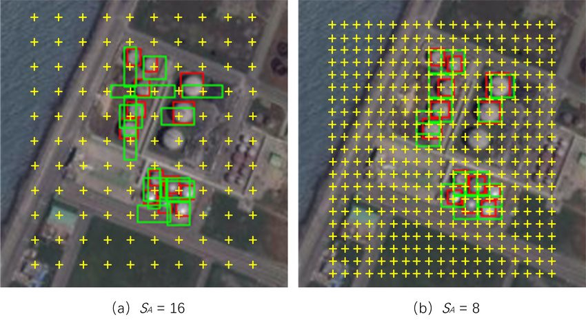
At each anchor point, there will be \(k\) predifined boxes in the original image

actually it doesn't matter where it lands.

If anchors are defind and refined with the coords on the feature map, then there should be one more step of back projecting them to the original image.

there are \(H\times W\) anchor points in the feature map, hence \(k \times H \times W\) anchors totally.

And there will be a set of predefined anchors in the original image \(I\) at every stride \(\mathcal{R}\).

Train RPN

1. determine loss

how assign ground truth to anchors during training

some are kept, a lot are abandoned.

• a single ground-truth box may assign positive labels to multiple anchors.

We assign a positive label to two kinds of anchors: (i) the anchor/anchors with the highest Intersection-over- Union (IoU) overlap with a ground-truth box, or (ii) an anchor that has an IoU overlap higher than 0.7 with 5 any ground-truth box. Note that a single ground-truth box may assign positive labels to multiple anchors.

Usually the second condition is sufficient to determine the positive samples;
but we still adopt the first condition for the reason that in some rare cases the second condition may find no positive sample.

We assign a negative label to a non-positive anchor if its IoU ratio is lower than 0.3 for all ground-truth boxes. Anchors that are neither positive nor negative do not contribute(abandoned) to the training objective.

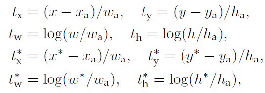
• a set of bounding-box regressors k are learned.

To account for varying sizes, a set of k bounding-box regressors are learned.

Each regressor is responsible for one scale and one aspect ratio, and the k regressors do not share weights

• Loss = cls + reg
  • as in Fast-RCNN

2. sampling

We follow the image-centric sampling strategy from [2] to train this network.

Each mini-batch arises from a single image that contains many positive and negative example anchors.

randomly sample 256 anchors in an image to compute the loss function of a mini-batch, where the sampled positive and negative anchors have a ratio of up to 1:1.

If there are fewer than 128 positive samples in an image, we pad the mini-batch with negative ones.

3. training strategy

refer to 3.2 Sharing Features for RPN and Fast R-CNN in the paper

first train RPN,
and use the proposals to train Fast R-CNN.
The network tuned by Fast R-CNN is then used to initialize RPN, and this process is iterated. This is the solution that is used in all experiments in this paper.

Why Faster?

Using RPN yields a much faster detection system than using either SS or EB because of shared convolutional computations; the fewer proposals also reduce the region-wise fully-connected layers’ cost

extract feature from a one-pass CNN feature map

Why using NMS?

One Point has many corresponding Prior-guided Anchors

NMS is performed after RPN

To reduce redundancy, we adopt non-maximum suppression (NMS) on the proposal regions based on their cls scores.

As we will show, NMS does not harm the ultimate detection accuracy, but substantially reduces the number of proposals.

After NMS, we use the top-N ranked proposal regions for detection.