博弈论算法 CFR算法

扩展性博弈与 CFR算法

扩展性博弈与 CFR算法
CFR算法的发展
扩展型博弈——知识回顾
Background
CFR 算法
- CRF算法的四个步骤
- 伪代码
CFR+
MCCFR

CFR算法的发展

算法

算法	鲁棒采样变体	神经网络变体	后悔值	后悔值匹配	策略更新	收敛速度	解概念	发表	时间
CFR：Regret Minimization in Games with Incomplete Information (neurips.cc)							NE	NIPS	2007
MCCFR:OS-MCCFR/ES-MCCFR: Monte Carlo Sampling for Regret Minimization in Extensive Games (neurips.cc)	√						NE	NIPS	2009
CFR+：Heads-up limit hold’em poker is solved Science				√			NE	Science	2015
CFVnets DeepStack: Expert-level artificial intelligence in heads-up no-limit poker		√	√				NE	Science	2017
VR-MCCFR：Variance Reduction in Monte Carlo Counterfactual Regret Minimization (VR-MCCFR) for Extensive Form Games Using Baselines	√						NE	AAAI	2019
LCFR:Solving Imperfect-Information Games via Discounted Regret Minimization Proceedings					√		NE	AAAI	2019
DCFR: Deep Counterfactual Regret Minimization (mlr.press)		√					NE	PMLR	2019
CFR-S :Learning to Correlate in Multi-Player General-Sum Sequential Games						√	CCE	NIPS	2019
CFR-Jr :Learning to Correlate in Multi-Player General-Sum Sequential Games						√	CCE	NIPS	2019

应用

主题	Paper	学校	发表	时间
无限注德州扑克	DeepStack:DeepStack: Expert-level artificial intelligence in heads-up no-limit poker	Alberta	Science	2017
无限注德州扑克	Libratus:Superhuman AI for heads-up no-limit poker: Libratus beats top professionals	CMU	Science	2018
六人无限注德州扑克	Pluribus:AI surpasses humans at six-player poker	CMU	Science	2019

强化学习的结合

主要内容	Paper	发表期刊	时间
采用反事实基线（counterfactual baseline）来解决信用分配的问题	COMA:Counterfactual Multi-Agent Policy Gradients	AAAI	2018
将后悔值融入行动器评判器（Actor-critic）的梯度更新过程，提出了无模型的多智能体强化学习方法后悔策略梯度	RPG:Actor-Critic Policy Optimization in Partially Observable Multiagent Environments	NIPS	2018
	AlphaHoldem:AlphaHoldem: High-Performance Artificial Intelligence for Heads-Up No-Limit Poker via End-to-End Reinforcement Learning	AAAI	2022

学习资料：

Learning, regret minimization, and equilibria[J] ：是cmu的讲义

Time and Space: Why Imperfect Information... | ERA (ualberta.ca): 是 stack 作者的博士论文 2017

Equilibrium Finding for Large Adversarial Imperfect-Information Game: Noam Brown 的博士论文 2020

基于状态抽象和残局解算的二人非限制性德州扑克策略的研究 - 中国知网 (cnki.net) ：哈工大（深研院）硕士论文 2017

基于实时启发式搜索的非完备信息博弈策略研究 - 中国知网 (cnki.net) : 哈工大（深研院）硕士论文 2018

[An Introduction to Counterfactual Regret Minimization](cfr.pdf (gettysburg.edu)) 本地

浅谈德州扑克AI核心算法：CFR - 掘金 (juejin.cn)

扩展型博弈——知识回顾

表示形式—— 博弈树

使用树状图来表示行动的次序和执行动作时的信息状态

图中有两个参与者，进行了两个阶段的博弈
结点：表示博弈的状态，
- 根节点：博弈的起点，玩家进行决策。关于博弈怎么开始，博弈的顺序，可以有预定的顺序也可以通过掷色子、投硬币决定等。
- 非叶子结点：决策结点：表示这个时候哪个博弈玩家做出决策。****
- 叶子结点：代表每个玩家在此时的收益。收益只存在于叶子结点
虚线框：信息集，同一信息集下可以执行的策略是一致的
实线、边：在此信息集下可以选择的策略，同一信息集下可以执行的策略是一致的
路径：从根结点到当前决策结点的路径中经过的决策的序列（有序集）

信息集 information set

以上虚线框就代表一个信息集。简单来说，虚线框下面的人不知道虚线框里的信息。也就是下一个玩家并不知道前一个玩家干了啥

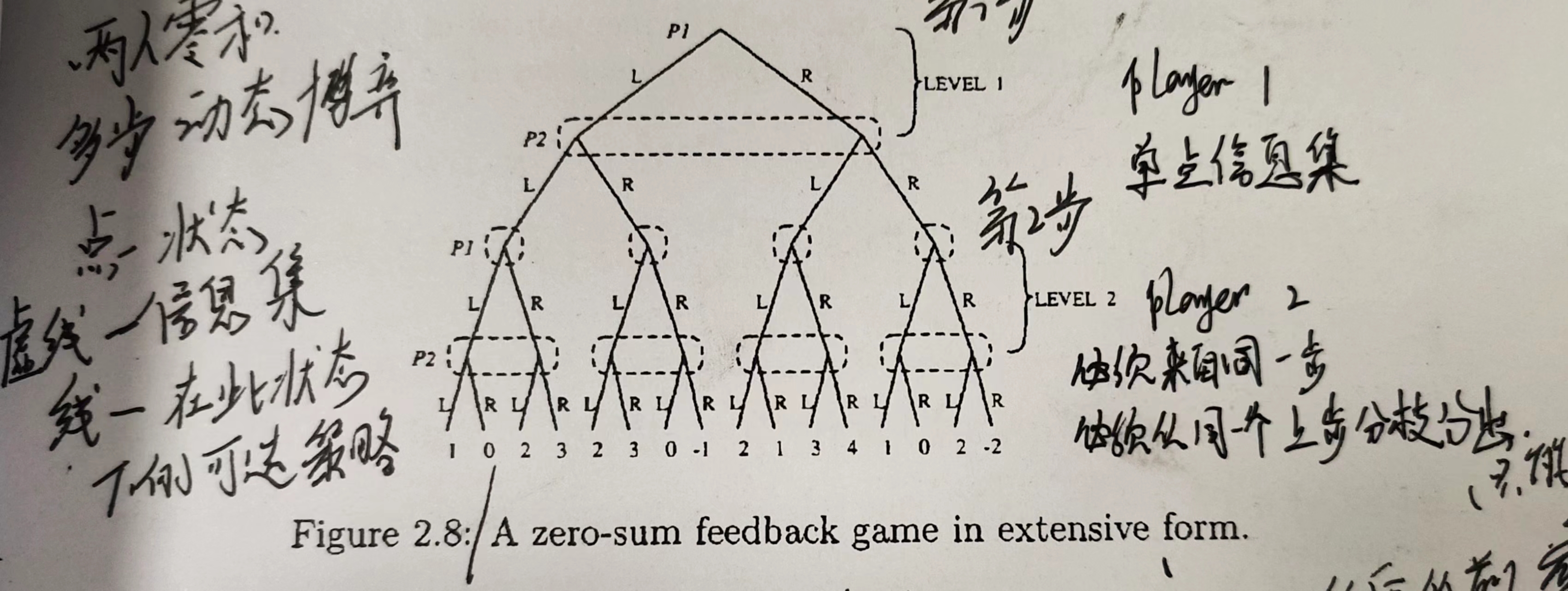
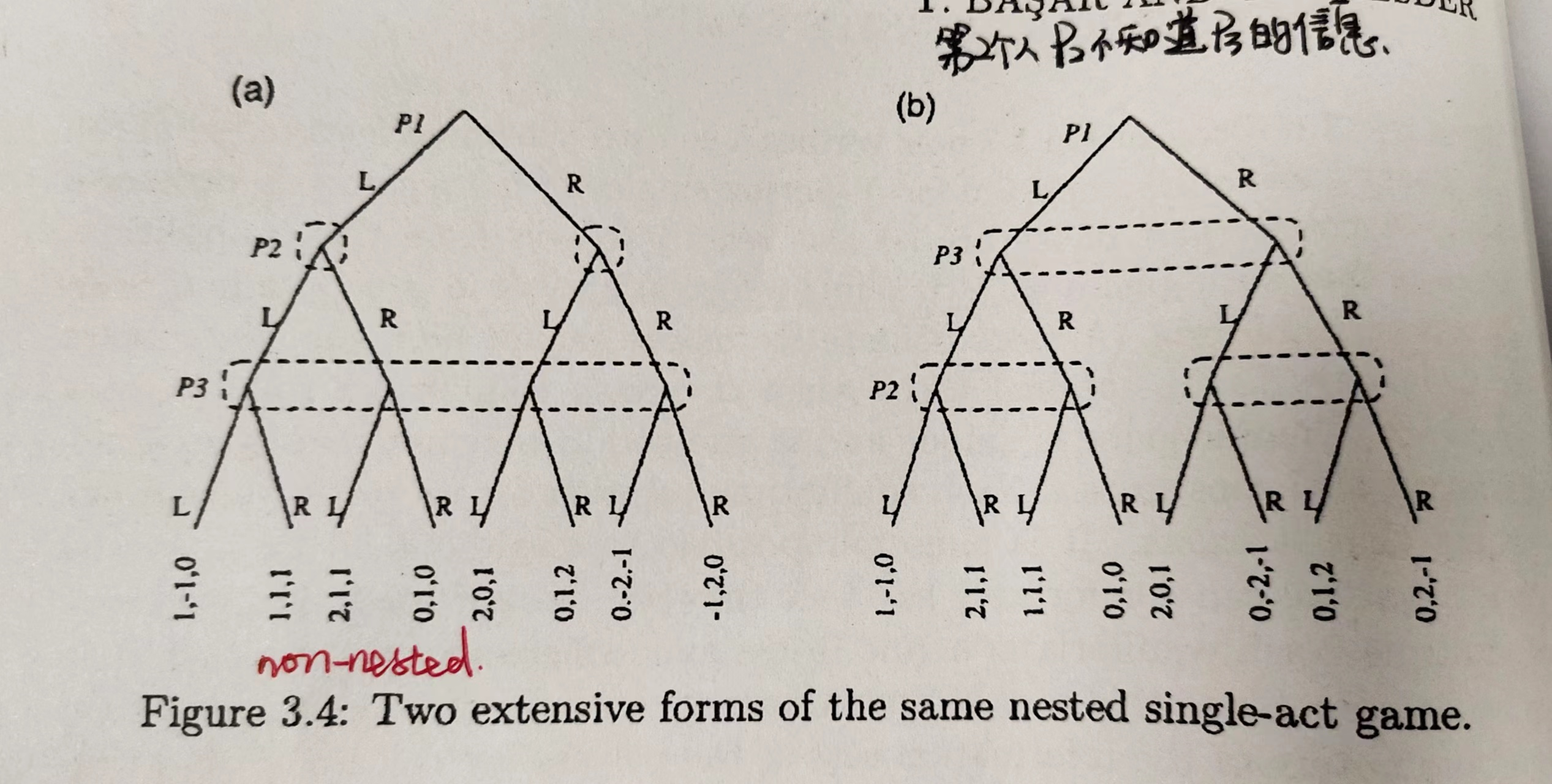
上图是一个二人单步行动的博弈。玩家P1 有两个可选行动，玩家P2有三个可选行动。P1先执行动作，P2后执行动作。收益是零和的，表示P2的收益，也就是P1的损失。

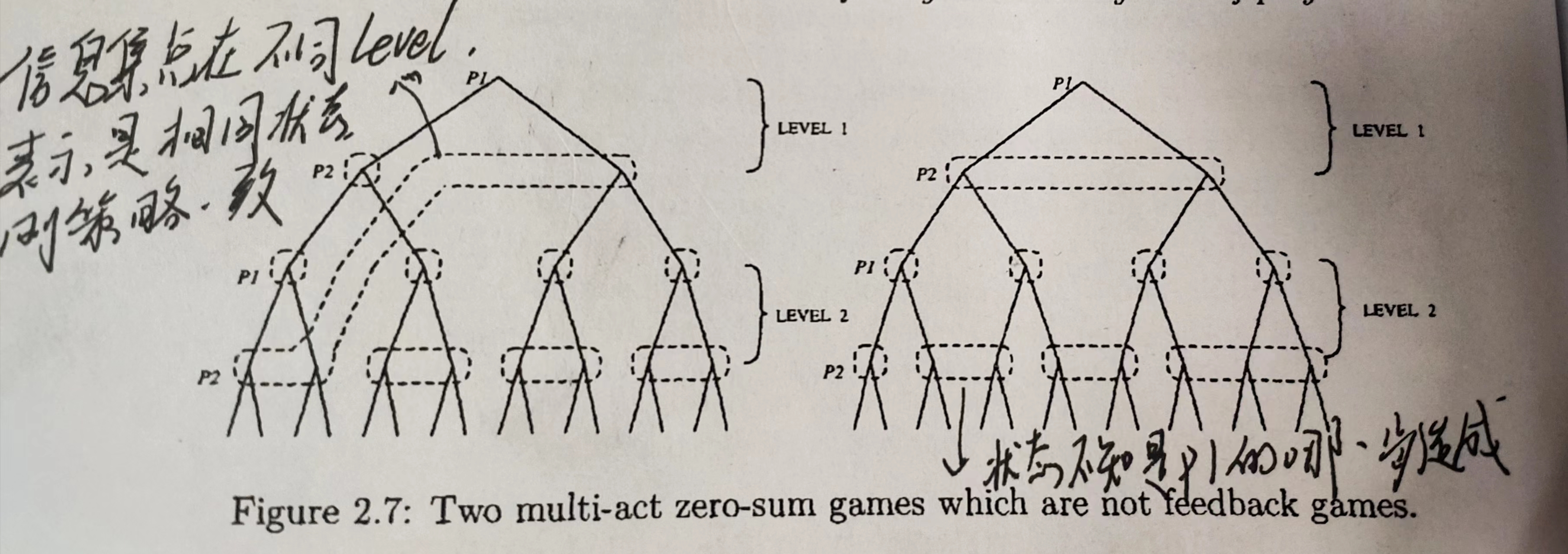
上图a和b的区别就只有信息集的不同。在图a中，P2的两个决策结点在同一个虚线框中，表示P2在决策的时候并不知道P1选择的动作及结果，即P2在决策并没有获得额外信息。在图b中，P2的决策结点在不同的虚线框中，因此P2观察到了P1选择了哪个行动，也就是从根节点到当前决策结点的路径是P2所知道的，此时P2有着完美信息。

完美信息与不完美信息
上图b清楚地表示了参与者1先动，参与者2观察到参与者1的行动。然而，有些博弈并不是这样，如图a所示，参与者并不是一直能观察到另一个人的选择(例如，同时行动或者行动被隐藏)。

信息集是决策节点的组合：
1、每个节点都属于一个参与者。
2、参与无法区分信息集里的多个节点。也就是说:如果信息集有多个节点，信息集所属的参与者就不知道能往哪个节点移动。

完美信息的博弈是指在博弈的任何阶段,每个参与者都清楚博弈之前发生的所有行动,也即每个信息集都是一个单元素集合。没有完美信息的博弈就是不完美信息博弈。

博弈树的公理化表述：

扩展性博弈研究范围的逐步扩展

二人零和单步 —— 二人非零和单步——多人非零和单步

二人零和多步——二人非零和多步——多人非零和多步

参与者：二——多
行动：单步——多步，有限——无限
收益：零和——非零和

有限二人零和多步动态博弈

有限：时间序列上有限，有中止结点

二人：两个参与者

零和：收益和为0

多步：多次采取行动

动态：有着信息集的概念，所谓的动态博弈，就体现在信息集的不唯一

1 feedback

图示

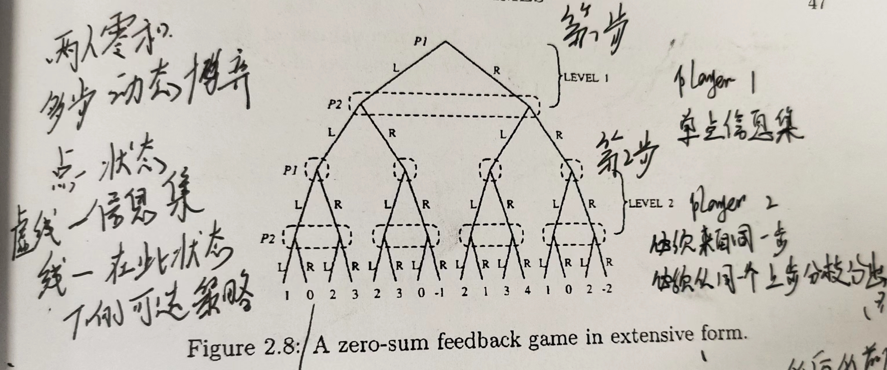
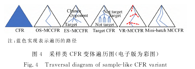
如上图2.8 所示的博弈为二人零和 feed back 博弈，需要满足两个条件：

每个参与者都有当前博弈阶段的完美信息。

从图中来看就是信息集都在同一层级，不会出现图2.7左边信息集跨越不同博弈阶段的情况；
每个阶段的博弈，后一玩家得信息集的结点不能来自前一玩家不同信息集结点的分支。

从图中来看就是，后面的信息集是从前一玩家的单个信息集延申出来的，如同图2.8所示，而不是2.7右边产生交叉的样子。

所以形如2.8所示的博弈树就是feedback型博弈，这样定义的目的是在之后的剪枝操作能够完全落下去。

求解saddle point 的方法

从最后的叶子结点，也就是最后一层开始，求解这一单步策略交互的鞍点均衡策略，计算收益值。将这一步的博弈剪枝操作，剪下来，用计算的均衡收益替换掉这个博弈树。

也就是将k步的博弈转换为k个1步的博弈。

2 openloop

图示

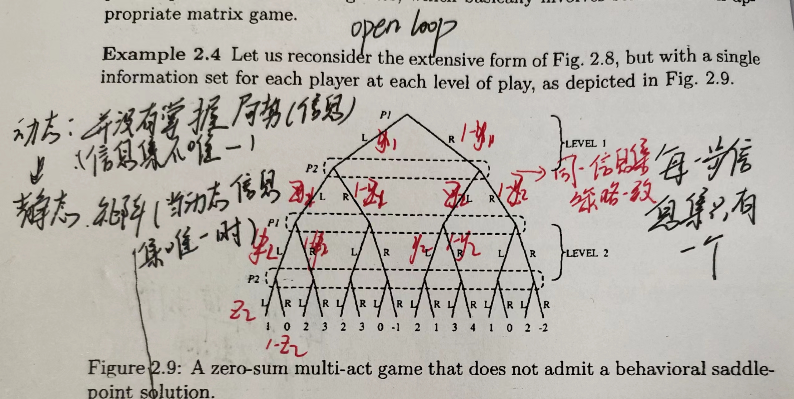
如上图所示，在博弈的每个阶段，所有决策结点都在同一个信息集中，这是一个完全的不完美信息博弈，也就是博弈的任何阶段,每个参与者都不清楚博弈之前发生的行动，这个时候也就没有任何额外的信息，其效果相当于一个静态博弈。

这种对于每个参与者每个阶段都只有一个信息集的博弈称之为 openloop型的扩展性博弈。

求解方法

由于信息集没有提供任何额外信息，其决策效果等同于博弈，所以可以将其多阶段的决策进行组合转换为一个单阶段的静态博弈。

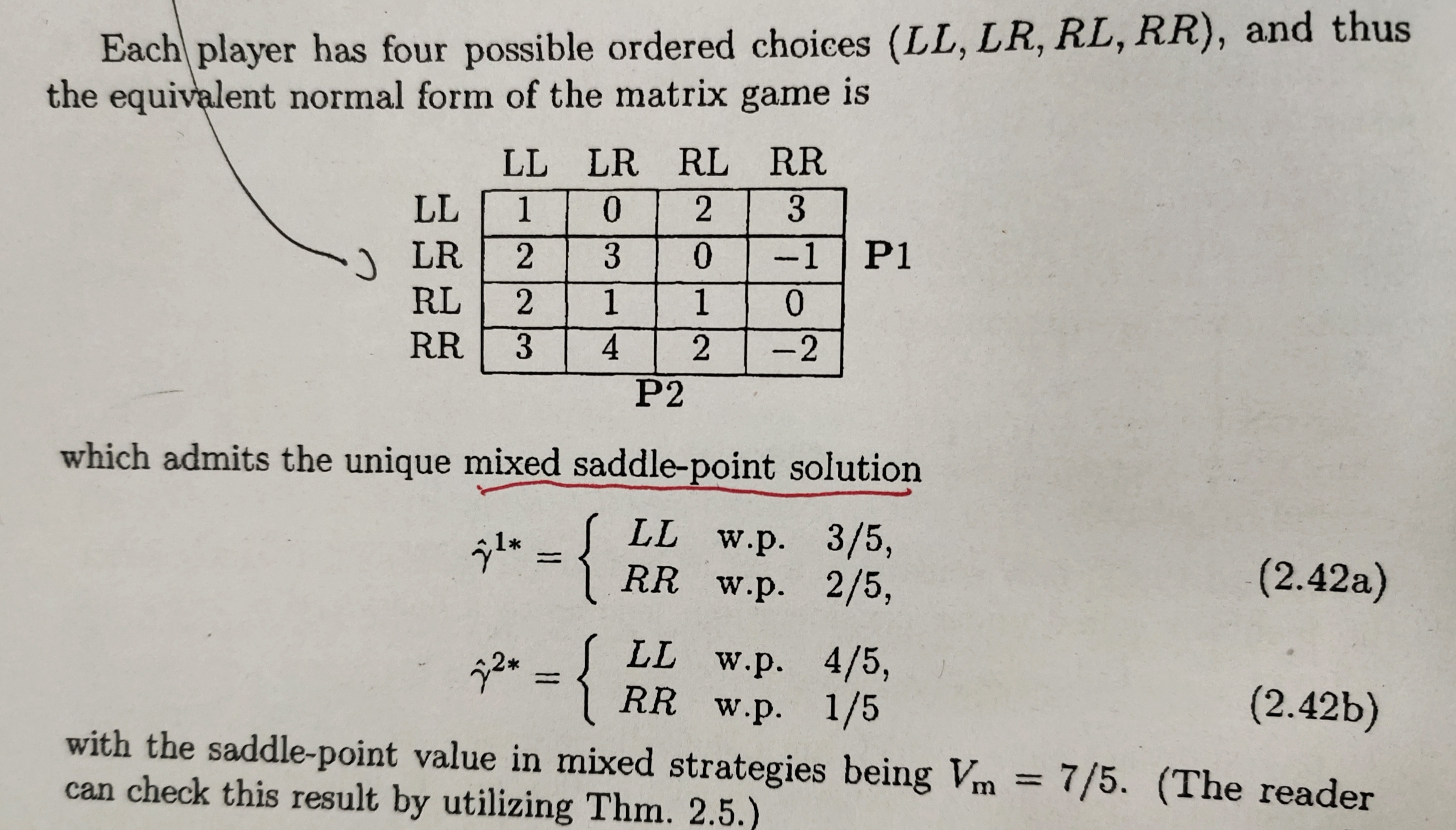
如将上图的openloop型博弈进行转换得到的标准型博弈矩阵如下，然后再求解其鞍点即可。

N 人博弈

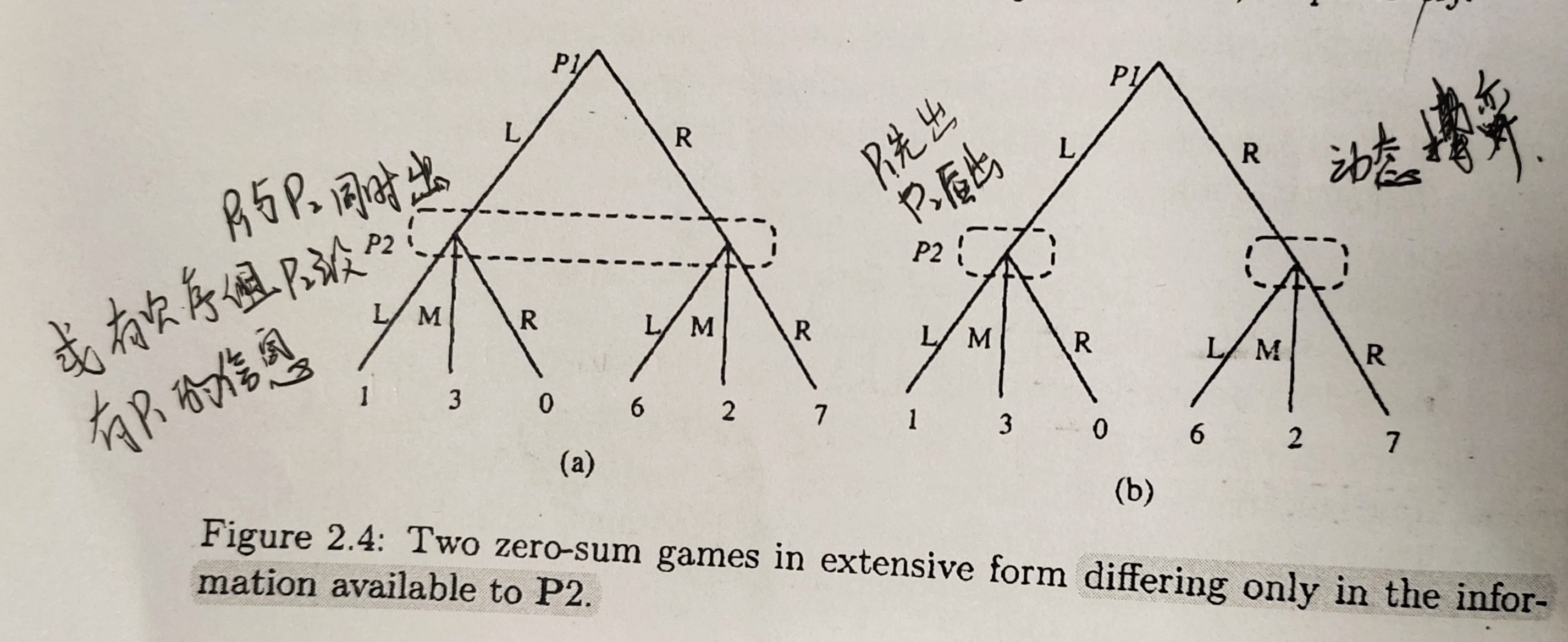
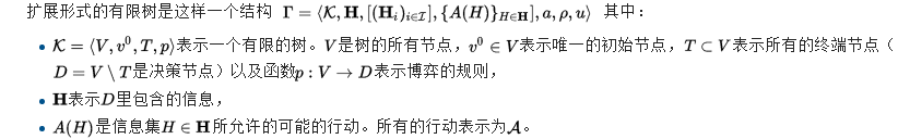
定义 Definition 3.10 extensive form tree structure

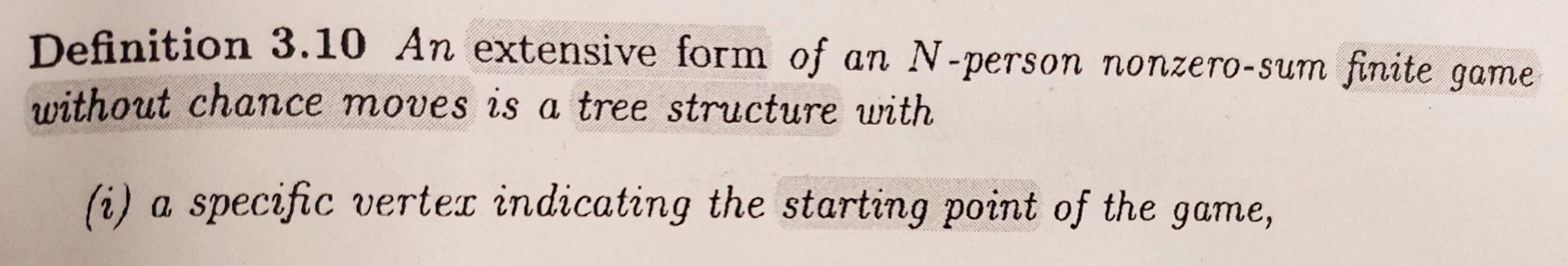
Definition 3.10 An extensive form of an N-person nonzero-sum finite game without chan moves is a tree structure with

a specific vertex indicating the starting point of the game

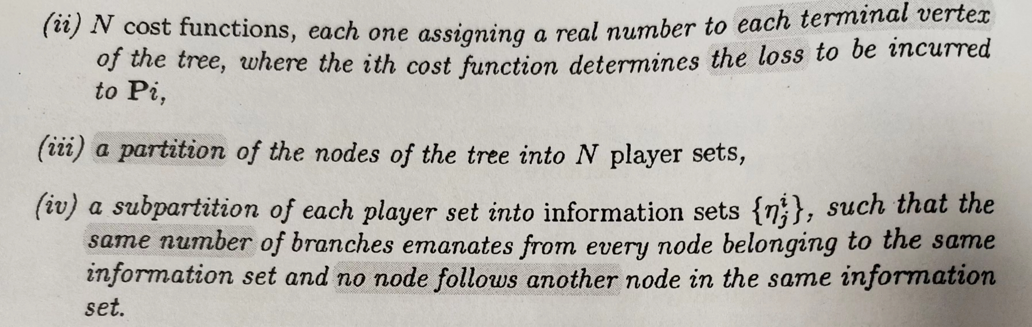
$N $ cost functions , each one assigning a real number to each terminal vertex of the tree,where the$ i$ th cost dunction determines the loss to be incurred to $P_i$。

a partition of the nodes of the tree into $N$ player sets

a subpartition of each player set into information sets $\{ \eta_j^i\}$，such that the same number of branches emanates from every node belonging to the same information set and no node follows another node in the same information set .

图示 Figure3.1

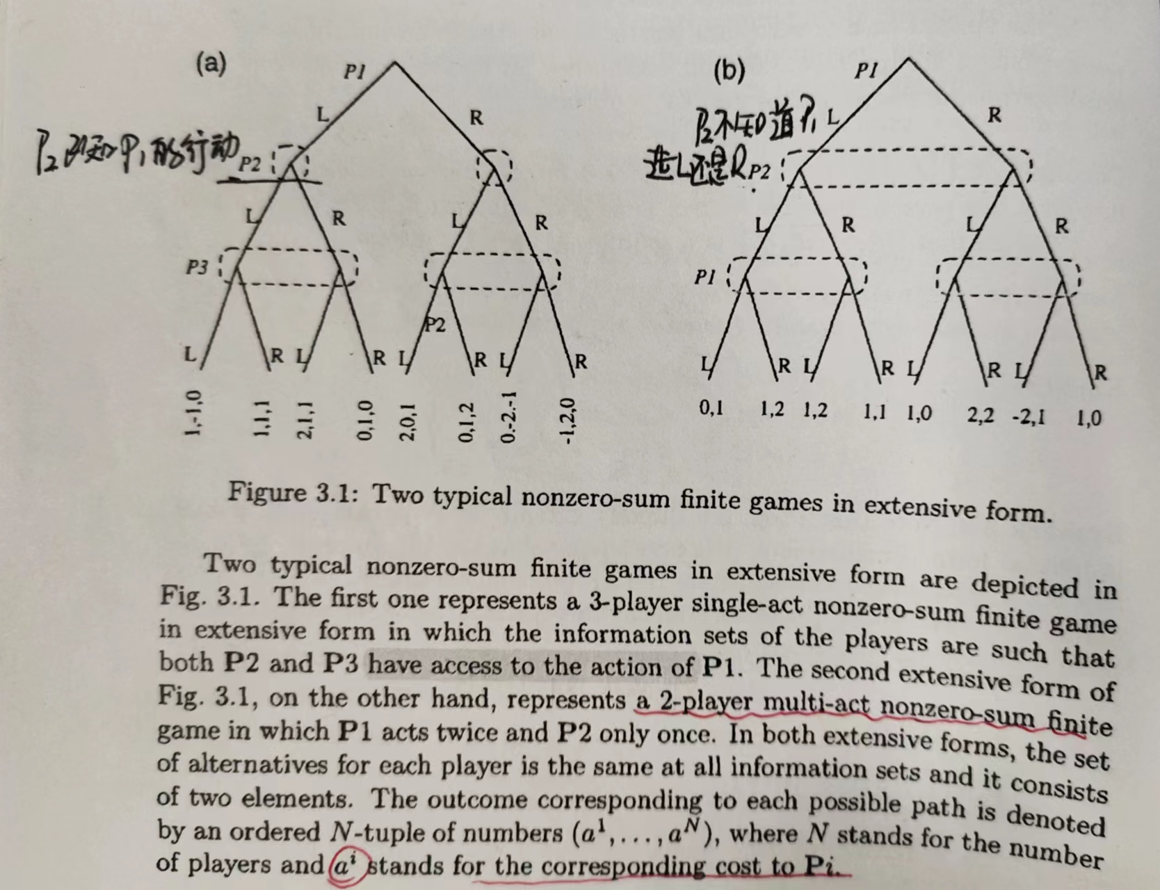
Two typical nonzero-sum finite games in extensive form are depicted in Fig. 3.1.

The first one represents a 3-player single act nonzero sum finite game in extensive form in which the information sets of the players are such that both P2 and P3 have access to the action of P1.

左边的图是三人单步博弈，P2,P3在决策结点都知道P1所采取的行动，但P3在决策的时候只知道P1的行动而并不知道P2的决策内容

The second extensive form of Fig. 3.1, on the other hand, represents a 2-player multi-act nonzero-sum fnite game in which P1 acts twice and P2 only once.

右边的图是二人多步博弈，其中P1有两次行动。在P2进行决策的时候并不知道P1的行动，P1第二次进行决策时知道自己第一步的行动但不知道P2的行动。

In both extensive formns, theset of alternatives for each player is the same at all information sets and it consise of two elements.

The outcome corresponding to each possible path is denotes by an ordered N-tuple of numbers $(a' .... aN)$, where$ N $stands for the number of players and a' stands for the corresponding cost to $P_i$.

单步博弈

图示 Figure3.2 3.3

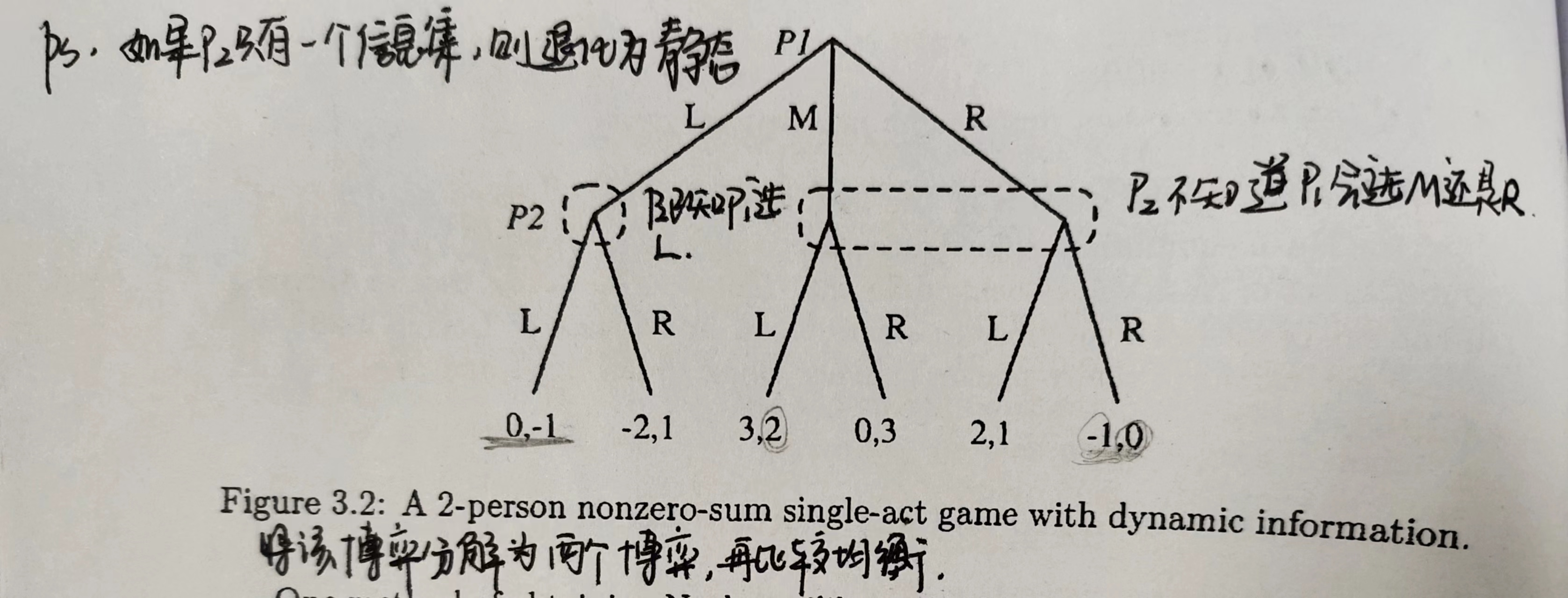
上图时二人单步博弈，P1先行动P2后行动，P1有3个可选择行动，P2有2个可选择行动。

重点关注一下信息集，在P2进行决策时候，如果P1选择行动L，那么P2在决策时是能够观察这个信息的；但如果P1选择行动M/R，这时候P2就不能确定是哪个，也就是这时候P2不知道P1选的是M/R，只知道P1没有选择L。

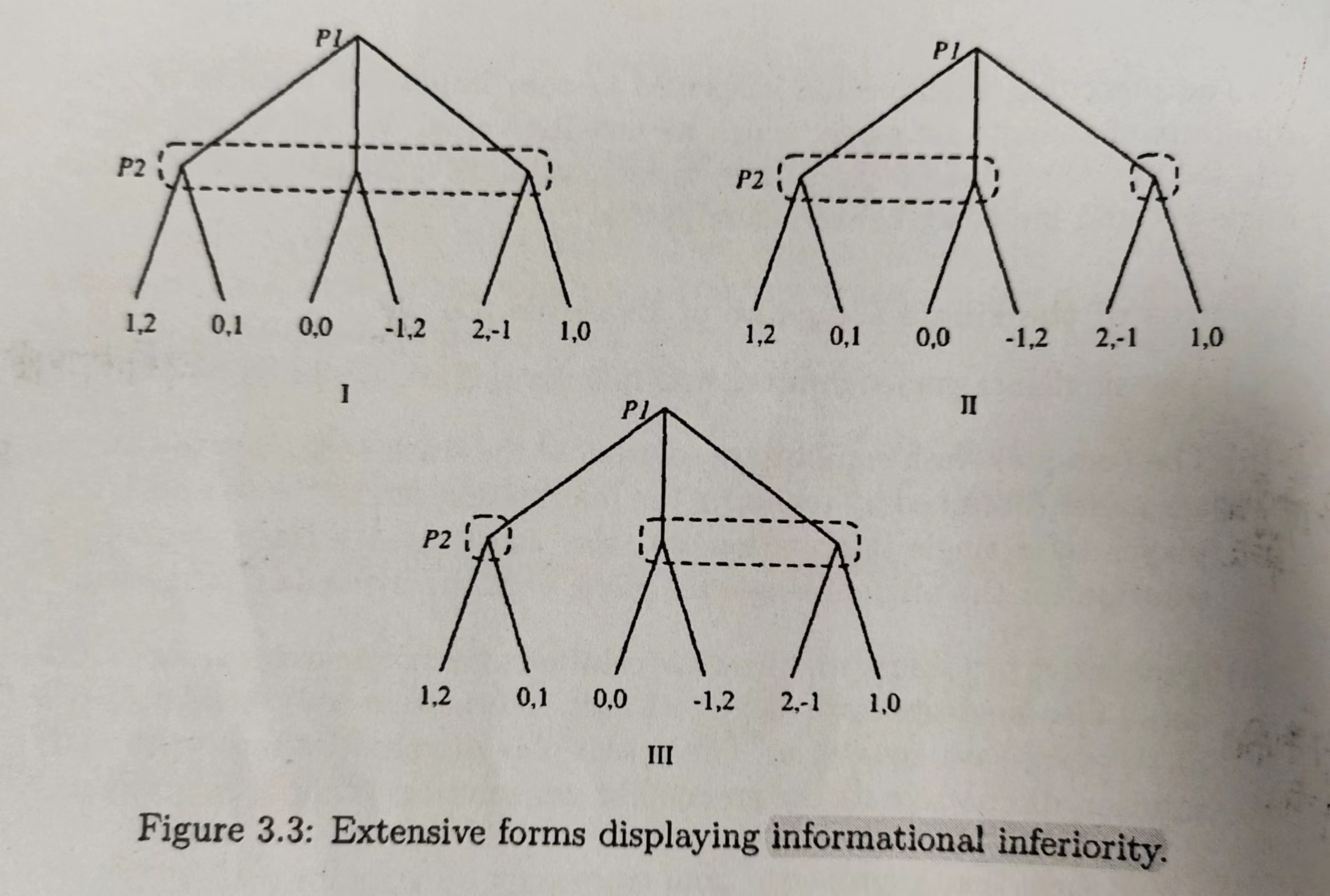
上图中三个差别就是在信息集的区别，显然，2和3与1相比，有着更多的信息。我们称博弈1信息低于2,3。而2，3之间并没有这种关系。

实际上，我们有博弈之间信息集“低于”的定义如下。

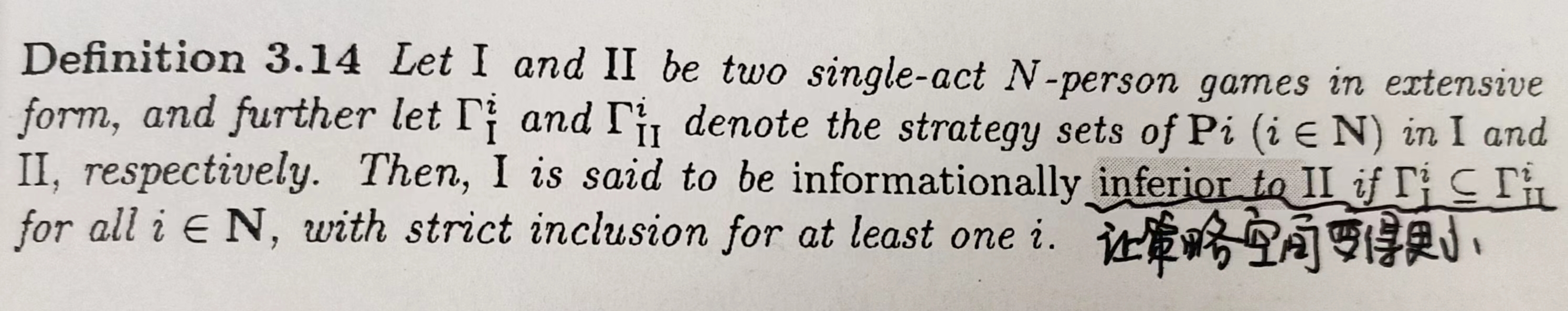
Definition 3.14 inferior

Definition 3.14 Let $I$ and $II$ be two single-act $N$-person games in extensive form ,and further let $ \Gamma_{\mathrm{I}}^{i} $ and $ \Gamma_{\mathrm{II}}^{i } $ denote the strategy sets of $P_i(i \in N)$ in $I$ and $II$ ,respectively. Then ,$I $ is said to be informationally inferior to $II$ if $ \Gamma_{\mathrm{I}}^{i} \subseteq \Gamma_{\mathrm{I}I}^{i}$ for all $i \in N$,with strict inclusion for at least one $i$.

两个博弈在均衡关系有以下定理。

Proposition 3.7 Let $I$ be an $N$-person single-act game that informationally inferior to some other single-act $N$-person game ,say $II$. Then

any Nash equilibrium solution of $I$ also constitues a Nash equilibrium solution for $II$,

if $\{\gamma^1,\cdots,\gamma^N\}$is a Nash equilibrium solution of $II$ so that $\gamma^i \in \Gamma^i_I$ for all $i \in N$ ,then it also constitues a Nash equilibrium solution for $I$

ladder-nested

定义 Definition 3.15 nested/ladder-nested

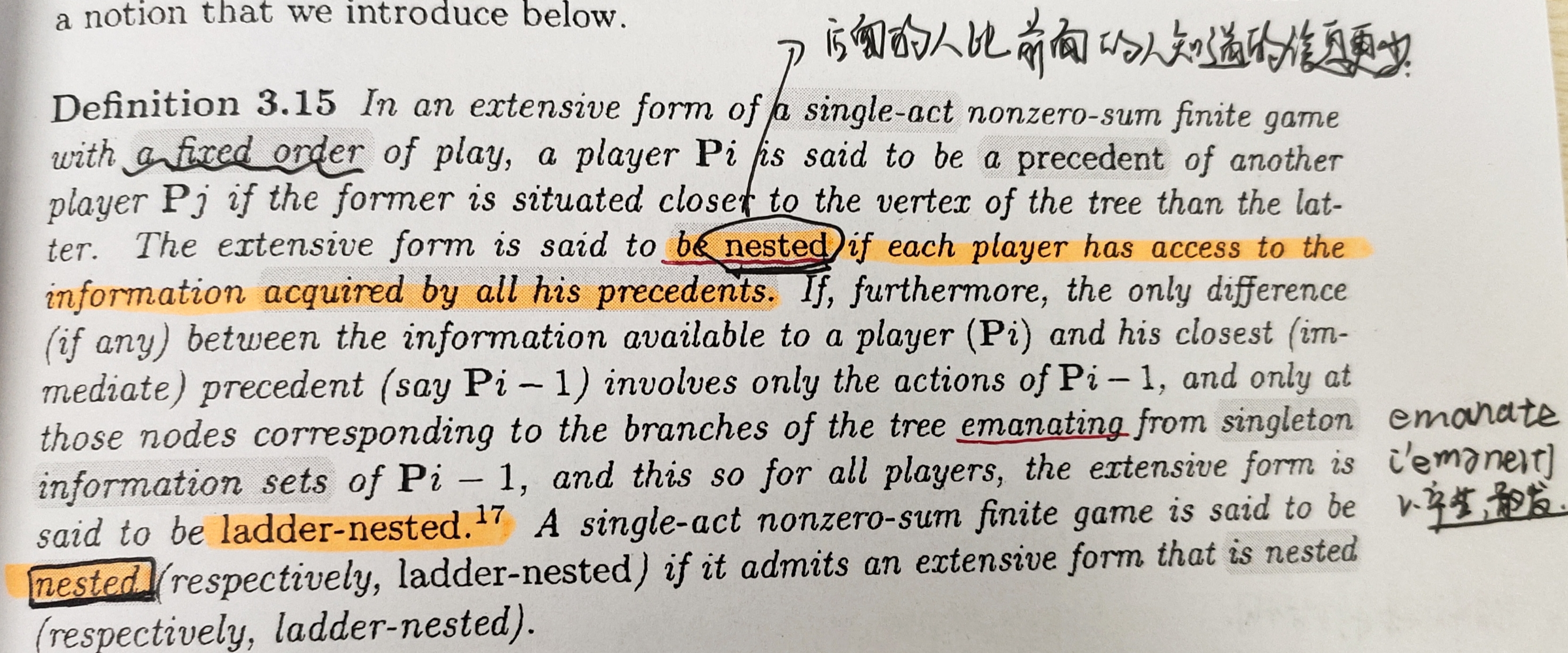
Definition 3.15

In an extensive form of a single act nonzero-sum finite game with a fixed order of play, a player $P_i$ is said to be a precedent of another player $P_j$ if the former is situated closet to the vertex of the tree than the latter.
The extensive forrm is said to be nested if each player has access to thei nformation acquired by all his precedents.

If, furthermore, the only diference(if any) between the information available to a player ($P_i$) and his closest (immediate) precedent (say $P_i - 1$) involves only the actions of $Pi- 1$, and only at those nodes corresponding to the branches of the tree emanating from singleton information sets of $P_i- 1$, and this so for all players, the extensiuve form is said to be ladder-nested.

A single- act nonzero-sum finite gameis said to be nested(respectively, ladder-nested) if it admits an extensive form that is nested
(respectively, ladder-nested).

17:Note that in 2-person single-act games the concepts of “nestednes" and "ladder-nstetes" coincide, and every extensive form is, by defnitin, ldder-nested

图示

Remark 3.7

The single act extensive forms of Figs. 3.1(a) and 3.2 are both ladder-nested.

If the extensive form of Fig. 3.1(a) is modified so that both nodes of P2 are included in the same information set, then it is only nested, but not ladder-nested, since P3 can differentiate between different actions of P1 but P2 cannot.

Finally, if the extensive form of Fig.3.1(a) is modified so that this time P3 has a single information set (see Fig. 3.4(a))， then the resulting extensive form becomes non-nested, since then even though P2 is a precedent of P3 he actually knows more than P3 does.

The single-act game that this extensive form describes is, however, nested since it also admits the extensive form description depicted in Fig. 3.4(b).

One advantage of dealing with ladder-nested extensive forms is that they can recursively be decomposed into simpler tree structures which are basically static in nature. This enables one to obtain a class of Nash equilibria of such games recursively, by solving static games at each step of the recursive procedure.
Before providing the details of this recursive procedure, let us introduce some terminology.

子集定义 Definition 3.16

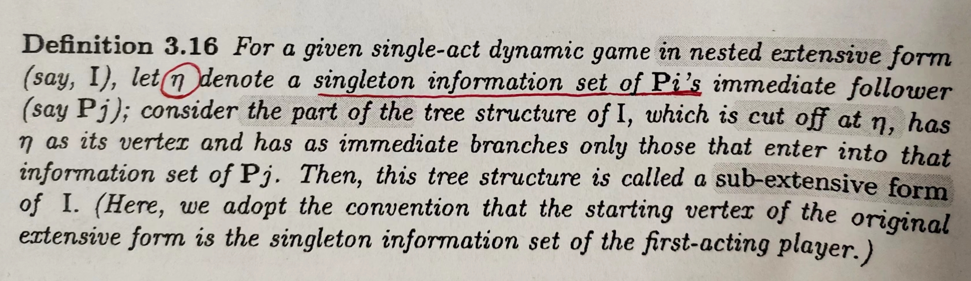
Definition 3.16

For a given single- act dynamic game in nested extensive forrm (say, $I$), let $\eta$ denote a singleton information set of $P_i$'s immediate follower (say $P_j$); consider the part of the tree structure of $I$, which is cut off at $\eta$, has $\eta$ as its vertex and has as immediate branches only those that enter into that inforrmation set of $P_j$.

Then, this tree structure is called a sub-extensive form of$ I$. (Here, we adopt the convention that the starting vertex of the original extensive form is the singleton inforrmation set of the first-acting player. )

拆解1 将ladder-nested 拆解为静态的

Definition 3.17

A sub-extensive form of a nested extensive form of a single-act game is static if every player appearing in this tree structure has a single information set.

图示：

Remark 3.8 The single act game depicted in Fig3.2 admits two sub-extensive forms which are as follows:

The extensive form of Fig. 3.1(a)， on the other hand, admits a total of for sub-extensive forms which we do not display here. It should be noted that each sub-extensive form is itself an extensive form describing a simpler game. The first one displayed above describes a degenerate 2-player game in which P1 has only one alternative. The second one again describes a 2-player game in which the players each have two alternatives. Both of these sub-extensive forms will be called static since the first one is basically a one player game and the second one describes a static 2-player game.

也就是说可以对信息集进行分解，将梯形结构拆解为简单的静态博弈。

下面给出一个例子

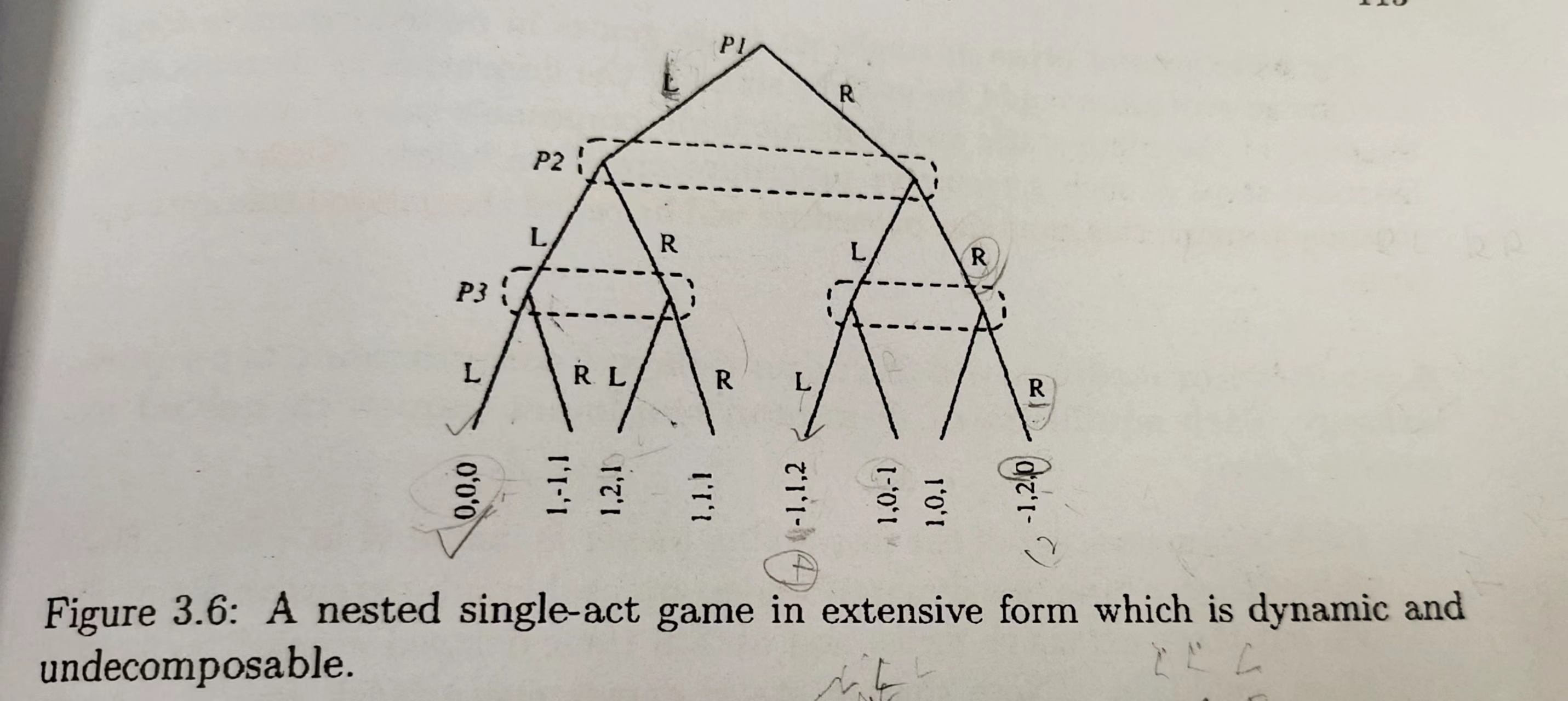
拆解2 将nested拆解为动态的 Definition 3.19

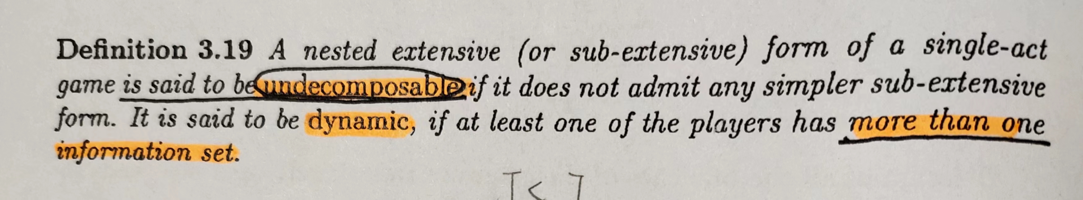
Definition 3.19 A nested extensive (or sub-extensive) form of a single-act game is said to be undecomposable if it does not admit any simpler sub-extensive form. It is said to be dynamic, if at least one of the players has more than one information set.

图示：

N人非零和feedback型的扩展型

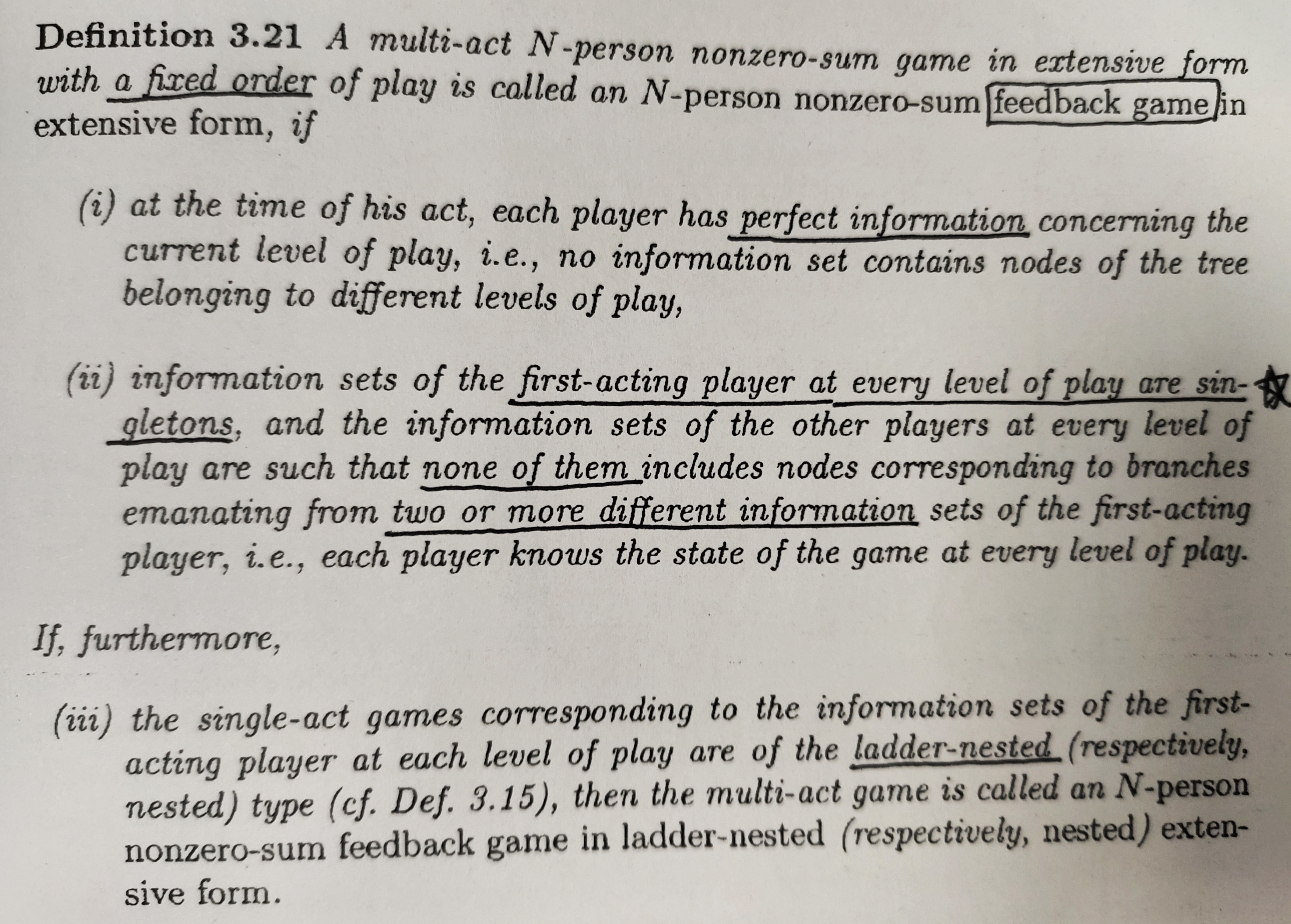
定义 Definition 3.21

Definition 3.21 A muiti-act N -person nonzero-sum game in extensive form with a fixed onder of play is called an N-person
nonzero-sum feedback game Jin extensive form, if

at the time of his act, each player has perfect information concerning the current level of play, i.e.,no information set contains nodes of the tree belonging to different levels of play,

information sets of the first- acting player at every level of play are singletons, and the information sets of the other players at every level of play are such that none of them includes nodes corresponding to branches emanating from two or more different information sets of the first-acting player, i.e., each player knows the state of the game at every level of play.

If, furthermore,

the single-act games corresponding to the information sets of the first-acting player at each level of play are of the ladder-nested (respectively nested) type (cf. Def. 3.15), then the multi-act game is clled an N-person nonzer-sum fedack game in ladder nested (eseptivele, neste) extensive form.

Background

扩展型博弈 Extensive Form Games

an extensive form game $G$ is a tuple $ \left\langle H, Z, P, p, u, \mathcal{I}, \sigma_{c}\right\rangle $.

$H$ is a set of states, including $\empty$, the initial state of the game. A state can alsobe called a history, because a game state is exactly history of the sequence of actions taken from the initial state. I will use $\cdot$ to indicate concatenation,so $h\cdot a$ is the sequence of actions in $h$, followed by action $a$.

$H$ :状态序列的集合

对于任何一个在集合$H$中的序列$h$，它是一个在某一次游戏中发生状态的序列，将此次博弈中发生的所有动作按照时间先后依次排列起来即得到$h$。从博弈树的角度来讲，$h$是从根节点到达博弈树中任意某个节点的路径。基于此我们可以做如下定义：$ h⊑j$ 表示$h$是$j$的子串， $h⊏j$ 表示$h$是$j$的真子串。对应到博弈树中则表示$j$是$h$的一个孩子节点。

图1表示的是德州扑克中的一个包含动作和状态的序列，箭头下方的字符表示每个玩家做出的动作，小写字母表示玩家1的动作，大写字母表示玩家2的动作，描述牌型的字符串是机会玩家的动作（可理解为发牌员做出的动作）。字母c是call动作的缩写，字母b是bet动作的缩写。

在图1中，状态h5为状态h6的子串，状态h6是状态h5在博弈树中的孩子节点；状态h1为状态h2、h3、h4、h5、h6的子串，状态h2、h3、h4、h5、h6都是状态h1在博弈树中的孩子节点。
$Z \subset H$ is the set of terminal (leaf) states, and $ u_{p}: Z \mapsto \mathbb{R} $ gives the payoff to player p if the game ends at state $z$.

$Z$: 终止状态的集合（对应博弈树中的叶子节点）

$u$：一个由终止状态到实数的映射，$u_p$表示某个玩家$p$到达终止状态$z$时可以获得的奖励
$P$ is a set of all players acting in the game,

$P$：参与游戏的所有玩家的集合

and $ p: H \backslash Z \mapsto P $ is a function which describes which player is currently acting at a non-terminal state $h$.

$p$：一个非终止状态到$P$中某一玩家的映射，表示当前状态应该由哪位玩家采取行动

The actions available at a non-terminal state $ h$ are defined implicitly by the set of histories $H$, so that $ A(h)={a \mid h \cdot a=j, h \in H, j \in H} $.

注意这个 $ h\cdot a$的表达 :表示在状态$h$上采取动作$a$

For a history $h$ where a stochastic event is about to happen, like a die roll or card deal, $p(h)$ is a special“ chance player” $c$. The value $ \sigma_{c}(h, a) $ gives the probability of chance event $ a$ occurring if the game is in state $h$.

$σ_c$：机会玩家（可理解为发牌员）做出所有合法动作的概率分布，可进一步用 $σ_c(h,a)$ 来表示当游戏处于状态$h$时，机会事件$a$发生的概率
$ \mathcal{I} $ describes what information is hidden from the players in a game, defined by a partition of all non-terminal, non-chance states.

$ \mathcal{I} $ must satisfy the constraints that $ \forall I \in \mathcal{I}$and $ \forall h, j \in I $, we have $p(h)= p(j)$ and $A(h)= A(j)$.

A set $I \in \mathcal{I}$ is called an information set, and for every state $h \in I$ the player $p(h)$ will only know that the current state of the game is one of the states in$ I$, but not exactly which one.

$I$：玩家的信息集，一个信息集中包含了若干个$H$中的状态，当其他玩家通过观测历史$h$时，只知道玩家处于集合$I$上，但是并不清楚该玩家具体在$I$的哪一个状态上。可以利用信息集的大小来衡量一个玩家在游戏中隐藏了多少信息

玩家策略

策略的描述

A player’s strategy, also known as their policy, determines how they choose actions at states where they are acting .The term strategy profile is used to refer to a tuple consisting of a strategy for each player.

策略是玩家在游戏中选择动作的准则，在非完备信息博弈中，策略$σ$是一个从当前信息集$I$上所有合法动作到$[0,1]$之间的一个映射，也可以说$σ$是一个基于信息集$I$的动作的概率分布

I will use $\sigma_p$ to refer to a strategy for player $p$, and $\sigma$ to refer to a strategy profile .

Given a strategy profile$\sigma$ and some player $p$ strategy $\sigma_p'$ , I will use the tuple $ <\sigma_{-p}, \sigma_{p}^{\prime}> $ to refer to the strategy profile where player $p$’s strategy is $\sigma_p'$, and their opponent plays according to their strategy in $\sigma$.

策略的概率 Strategy Probabilities

$ \sigma_{p}(I, a) $ gives the probability of player $p$ making action $a$ given they have reached information set$ I \in \mathcal{I}{p} $, and $ \sigma(I, a)=\sigma(I, a) $. I will use the vector $σ(I)$ to speak of the probability distribution $σ(I, a)$ over $A(I)$.

$ \sigma_{p}(I, a) $：玩家$p$处于信息集$I$时，做出动作$a$的概率

$σ(I)$：表示一个概率分布，即处于状态集$I$时，做出所有合法动作的概率分布（将游戏中所有的信息集$I$上的$ σ(I)$ 组合起来，即可得到完整的策略$σ$

$ \pi^{\sigma}(h) $ gives the probability of reaching state $h$ if all players follow profile $\sigma$.

$ \pi_{p}^{\sigma}(h) $ gives the probability of reaching state $h$ if chance and $p$’s opponents make the actions to reach $h$, and player $p$ acts according to $σ$.

We can also extend the $π$ notation by flipping which players are following $σ$ and use $ \pi_{-p}^{\sigma}(h) $ to refer to the probability of reaching state $h$ if player $p$ makes the actions to reach $h$, and chance and $p$’s opponents act according to $σ$.

All of these $π$ probabilities can also be extended to consider subsequences of actions. We can speak of $ \pi_{p}^{\sigma}(z \mid h) $ as the probability of player $p$ making the actions needed to move from state$ h$ to state $z$.

$ \pi^{\sigma}(h) $ ：从初始状态出发，当所有玩家都遵循策略$σ$时，到达状态$h$的概率

$ \pi_{p}^{\sigma}(h) $ ：玩家$p$从初始状态出发，遵循策略$σ$，到达状态$h$的概率

$ \pi_{-p}^{\sigma}(h) $ ：从初始状态出发，除玩家$p$外，其他所有玩家都遵循策略$σ$，到达状态$h$的概率。

$ \pi_{p}^{\sigma}(z \mid h) $ ：玩家$p$遵循策略$σ$，从状态$h$出发，到达中止状态$z$的概率

关于$π$概率这一定义，有以下三个等式需要额外注意：

1． $ \pi^{{\sigma}(h)=\pi_{p}}(h) \pi_{-p}^{\sigma}(h) $ ：这个等式表明所有玩家遵循策略$σ$到达状态$h$的概率等于每个玩家分别遵守策略$σ$到达状态$h$的概率相乘；

这个式子是关于玩家的方向来看，多人游戏，想要到达某个状态不但取决于玩家$p$的策略

2． $ \pi_{p}^{\sigma}(I, a)=\pi_{p}^{\sigma}(I) \sigma(I, a) $：这个等式表明所有$π$概率都可以表示为一系列 $σ(I^k,a) $概率的乘积；

其中右边$\pi_{p}^{\sigma}(I)$代表玩家$p$从初始状态出发，遵循策略$σ$，到达到达信息集$I$的概率，$\sigma(I, a)$表示在信息集$I$下做出动作$a$的概率

左边的就表示代表玩家$p$从初始状态出发，遵循策略$σ$，到达到达信息集$I$，并做出动作$a$的概率

3． $ \pi^{{\sigma}(z)=\pi}(h) \pi^{\sigma}(z \mid h) $ ：这个等式是等式2的推论，表明从初始状态出发，遵循策略$σ$到达状态$z$的概率等于从初始状态出发，遵循策略$σ$到达状态$h$（h是z的子串）的概率乘以遵循策略$σ$，从状态$h$出发到达状态$z$的概率。

这个式子是从路径的长度来看的，总路径$0-z$和中间结点$0-h,h-z$的关系

策略的价值 Strategy Values

接下来基于终止状态的收益$u$对博弈树中的每个节点都定义一个收益。

最主要的目的是给出博弈树中的中间非叶子结点的收益。

当玩家$p$遵循策略$σ$时，对于博弈树中任意的一个状态$h$，该状态的收益定义为：

\[u_{p}^{\sigma}(h)=\sum_{z \in Z, h \sqsubset z} \pi^{\sigma}(z) u_{p}(z) \]

式子中，$u_p(z)$ 按着前面的定义即为玩家$p$到达终止状态$z$（叶子节点）所获得的收益；

前面的$\pi^\sigma(z)$表示从初始状态出发，当所有玩家都遵循策略$σ$时，到达终止状态$z$的概率；

求和即表示从初始状态开始把所有包含路径$h$到达终点$z$的序列进行求和

这个收益即表示玩家$p$ 从博弈起点到中间状态$h$ 再根据策略$\sigma$到达终点$z$得到的收益。

可以将右端前一项根据概率式1 进行拆分，得到

\[\begin{aligned} u_{p}^{\sigma}(h) &=\sum_{z \in Z, h \sqsubset z} \pi^{\sigma}(z) u_{p}(z) \\ &=\sum_{z \in Z, h \sqsubset z} \pi_{p}^{\sigma}(z) \pi_{-p}^{\sigma}(z) u_{p}(z) \ 参与者拆分(1) \\ &=\sum_{z \in Z, h \sqsubset z} \pi^{\sigma}(h) \pi^{\sigma}(z \mid h) u_{p}(z) \ 路径拆分(3) \\ &=\pi_{p}^{\sigma}(h) \sum_{z \in Z, h \sqsubset z} \pi_{-p}^{\sigma}(h) \pi^{\sigma}(z \mid h) u_{p}(z) 参与者+路径拆分(1)+(3) \end{aligned} \]

根据此定义，整局游戏的收益即为博弈树根节点的收益 $ u_{p}^{{\sigma}=u_{p}}(\varnothing) $

对于这个定义，需要留意的是：除根节点外，状态h的收益并不是从状态h出发，可以到达的所有终止状态收益的期望。若用期望作为收益，收益的形式化定义应该是这样的：$u_{p}^{\sigma}(h)=\Sigma_{z \in Z, h \sqsubset z} \pi^{\sigma}(z \mid h) u_{p}(z)$

理解为什么要使用上面的等式来作为状态$h$的收益：状态$h$的收益是基于玩家采用的策略$σ$的，同一局游戏采用不同的$σ$会产生不同的动作序列，进而产生不同的收益。若我们使用下面的等式作为状态$h$的收益，那么我们对到达状态$h$之前遵循的策略则没有做出约束，到达$h$之后才会一直遵循策略$σ$，在$h$之前采用的策略是随机的。这显然不符合实际情况。

当玩家$p$遵循策略$σ$时，对于博弈树中的一个信息集$I \in \mathcal{I}$的收益定义为：

\[ u_{p}^{\sigma}(I)=\sum_{h \in I} u_{p}^{\sigma}(h) \]

反事实值 the counterfactual value

Counterfactual value differs from the standard expected value in that it does not consider the player s own probability of reaching the state (thus the use of counterfactual in the name: instead of following σ, what if the player had instead played to reach here?)

反事实值不同于标准期望值，因为它不考虑玩家自己达到状态的概率(因此在名称中使用反事实: 如果不遵循策略σ，如果玩家到达这里的概率是怎么样的?)

The counterfactual value for player$ p$ of state $h$ is

\[v_{p}^{\sigma}(h)=\sum_{z \in Z, h \sqsubset z} \pi_{-p}^{\sigma}(h) \pi^{\sigma}(z \mid h) u_{p}(z) \]

看这个式子的定义：

右端第一项$\pi_{-p}^{\sigma}(h)$ 表示其他玩家$-p$选择策略$\sigma$ 从起点到达中间结点$h$的概率；

第二项$\pi^{\sigma}(z \mid h)$ 表示路径经过中间结点$h$，然后根据策略$\sigma$到达最终结点$z$的概率，

右端第三项表示玩家$p$在最终结点$z$的收益，然后对所有经过中间结点$h$到达最终结点$z$的路径进行求和。

~~但我们知道想要根据策略$\sigma$从博弈起点到达最终结点$z$，玩家$p$也要根据策略$\sigma$ 从起点到达中间状态$h$,但上面式子缺失了这一块~~

~~反事实值也就表示，不遵循策略$\sigma$的时候从起点到达中间状态$h$的收益；~~

~~反事实值越大，表示不遵循策略$\sigma$是好的；~~

~~当遵循$\sigma$时候，反事实越大，越不可能到达$h$状态。~~

结合第2小节中关于$π$概率的三个等式，我们可以很容易地推导出状态$h$的收益值与反事实值之间的关系：

\[\begin{aligned} u_{p}^{\sigma}(h)&=\Sigma_{z \in Z, h \sqsubset z} \pi^{\sigma}(z) u_{p}(z) \\ &=\Sigma_{z \in Z, h \sqsubset z} \pi^{\sigma}(h) \pi^{\sigma}(z \mid h) u_{p}(z) \\ & =\Sigma_{z \in Z, h \sqsubset z} \pi_{p}^{\sigma}(h) \pi_{-p}^{\sigma}(h) \pi^{\sigma}(z \mid h) u_{p}(z) \\ & =\pi_{p}^{\sigma}(h) \Sigma_{z \in Z, h \sqsubset z} \pi_{-p}^{\sigma}(h) \pi^{\sigma}(z \mid h) u_{p}(z) \\ & =\pi_{p}^{\sigma}(h) v_{p}^{\sigma}(h) \\ \end{aligned} \]

上述等式不仅揭示了收益值和反事实值之间的关系，而且还解释了反事实值的实际意义：

对于某个玩家$p$，遵循特定策略$σ$到达状态$h$，在此策略指导下到达状态$h$的概率越小，则其相应的反事实值越大；在此策略指导下到达状态$h$的概率越大，则其相应的反事实值越小。

当在策略$σ$下到达状态$h$的概率为$1$时，反事实值和收益值相等。

总结起来就是，在遵循策略$σ$时，反事实值的大小和到达状态$h$的可能性成反比。在策略$σ$下，越不可能到达$h$状态，该状态越反事实。

同样的，将概念扩展到信息集上有 the counterfactual value for player $p $ of an information set $I \in \mathcal{I}_p$ is

\[v_{p}^{\sigma}(I)=\sum_{h \in I} v_{p}^{\sigma}(h) \\ v_{p}^{\sigma}(I \cdot a)=\sum_{h \in I \cdot a} v_{p}^{\sigma}(h) \]

最优反应 Best Response

最佳反应和最佳反应收益是博弈论中很重要的两个概念，它们的形式化定义如下：

\[b r_{p}(\sigma)=\operatorname{argmax} \sigma_{\sigma^{*} \in \Sigma_{p}} u_{p}^{<\sigma_{-p}, \sigma *>} \\ v b r_{p}^{\sigma}=\max _{\sigma^{*} \in \Sigma_{p}} u_{p}^{<\sigma_{-p}, \sigma *>}=u_{p}^{<\sigma_{-p}, b r_{p}(\sigma)>} \]

上述定义符号有些复杂，我们用自然语言来解释一下上述定义：最佳反应是一种策略，使用这种策略可以在其他玩家都使用策略$σ$时获得最大收益，使用最佳反应策略获得的收益值即为最佳反应收益。

最佳反应是我们在已知对手策略时的最优选择，相应的，根据我们的策略推算对手的最佳反应也能够给出我们目前策略下最坏情况的参考。

策略空间 Strategy Space

Behaviour Strategies

A behaviour strategy $σ_p$ directly specifies the probabilities $σ_p(I, a)$. When playing a game according to a behaviour strategy, at every information set $I$ the player samples from the distribution$ σ(I)$ to get an action.

Similar to sequence form strategies, the size of a behaviour strategy is $ \sum_{I \in \mathcal{I}_{p}}|A(I)| $.

The first down side of behaviour strategies is that the expected value is not linear in the strategy probabilities, or even a convex-concave function.

The second problem is that computing the average of a behaviour strategy is not a matter of computing the average of the specified action probabilities: it is not entirely reasonable to give full weight to a strategy’s action probabilities for an information set that is reached infrequently. Instead, to compute the average behaviour strategy we must weight $σ_p(I, a)$ by $π_p^σ(I)$, which is equivalent to averaging the equivalent sequence form strategies.

遗憾 Regret

遗憾的概念

Much of my work makes use of the mathematical concept of regret. In ordinary use, regret is a feeling that we would rather have done something else. The mathematical notion of regret tries to capture the colloquial sense of regret, and is a hindsight measurement of how much better we could have done compared to how we did do.

我的大部分工作都使用了遗憾的数学概念。在通常的用法中，后悔是一种我们宁愿做别的事情的感觉。

遗憾的数学概念试图抓住口头意义上的遗憾，是一种事后衡量，与我们做的相比，我们本可以做得更好多少。

Assume we have a fixed set of actions $A$, a sequence of probability distributions $σ^t$ over $A$, and a sequence of value functions $ v^{t}: A \mapsto \mathbb{R} $.

注解：While $A$ is fixed, both $σ_t$ and $v_t$ are free to vary over time.

虽然可选动作集 $A$ 是固定的，但策略$σ_t$ 和收益 $v_t$ 都可以随时间自由变化。

注意这里的$v^t$是动作集合上的收益值，其概念和定义与之前定义在某一状态的收益$u$ 以及定义在某一状态的反事实值$v_{p}^{\sigma}(h)$都不一样，这个定义更类似于即时奖励的概念所以这个文章在这一点上符号表达是有些混乱的，便于理解可以将其改为 r $r^t: A \rightarrow \mathbb{R} $

同样的，这里的$\sigma^t$就表示$t$时刻在动作集合$A$上的一个概率分布

Given some set of alternative strategies$ S$, where $s ∈ S$ maps time$ t ∈ [1...T]$ to a probability distribution $s(t)$ over$ A$, our regret at time $T$ with respect to $S$ is

\[R^{T}(s)=\sum_{t} s(t) \cdot v^{t}-\sum_{t} \sigma^{t} \cdot v^{t} \\ R^{T}(s)=\sum_{t} s(t) \cdot r^{t}-\sum_{t} \sigma^{t} \cdot r^{t} \]

The regret can then be written in terms of the choice regrets as

\[R_{S}^{T}=\max _{s \in S} R^{T}(s) \]

将我们实际使用的策略$σ$替换成策略$s$，新策略$s$比原策略多产生的那部分收益（即时奖励的和），即为遗憾值的数值。

这里的$\sigma^{t} \cdot v^{t}$的含义是？当前$t$时刻，在动作集合$A$上动作的概率分布（动作的选择，也就是策略，理解：石头剪刀布1/3,1/3,1/3 和1/2,1/2,0就是两种不同的策略）乘以动作的奖励，也就是当前时刻根据所采取的策略所得到的期望奖励。将策略（动作集合的分布概率）进行替换后会得到新的奖励的期望。两者的差别就是策略的选择（例如赌博，all in 还是压哪几个），也就产生了遗憾。

需要特别说明的是，遗憾值中的收益$r$可以是任意一个从动作集合$A$到实数$R$的映射（任意的动作的即时奖励），只需保证总累积遗憾值具有次线性，那么遗憾值就可以被最小化。

当所有动作都产生的遗憾值都足够小时，我们就可以认为我们的策略已经足够接近纳什均衡，问题得以解决。

所以遗憾也可以写为在所有可替换策略中使得遗憾值最大的那个，只要使得最大的遗憾值变得特别小即可。

遗憾的边界

In order for regret to be meaningful, we need bounded values, so that there is some$ L$ that $ \left|v^{t}(a)-v(b)\right| \leq L \forall t $ and $ \forall a, b \in A $.

为了能够进行数值表示，不同的动作的奖励值得差距不超过$L$倍

External Regret 外部遗憾

Using different sets $ S$ gives different regret measures.

The most common, external regret, uses $S$ such that $∀s ∈ S$, $s(t)$ is a probability distribution placing all weight on a single action $A$, and $∀t、 t′, s(t) = s(t′)$. That is, external regret considers how we would have done if we had always played a single, fixed action instead.

在遗憾最小化算法中，使用一种特殊的遗憾值：External Regret，即用一特定动作$a$代替当前策略，产生的遗憾值。

\[R^{T}(a)=\sum_{t} a \cdot v^{t}-\sum_{t} \sigma^{t} \cdot v^{t} \\ R^{T}(a)=\sum_{t} a \cdot r^{t}-\sum_{t} \sigma^{t} \cdot r^{t} \]
理解：所谓策略就是动作集合上概率的分布，选择特定的动作也就是比如原来的策略剪刀石头布的动作的选择概率分布为$1/3,1/3,1/3$,

改变策略可以有很多种可能性例如$1/2,1/2,0$等等，这个概念考虑将策略变为一个固定的动作的选择，也就是将剪刀石头布的动作的选择概率分布变为$0,0,1$

在线学习和遗憾值最小化 Online Learning and Regret Minimisation

在线学习问题

Let us say we have a repeated, online, decision making problem with a fixed set of actions. At each time step, we must choose an action without knowing the values in advance. After making an action we receive some value (also known as reward), and also get to observe the values for all other actions.The values are arbitrary, not fixed or stochastic, and might be chosen in an adversarial fashion.

The adversary has the power to look at our decisionmaking rule for the current time step before we make the action, but if we have a randomised policy the adversary does not have the power to determine the private randomness used to sample from the distribution.

This setting is often called expert selection, where the actions can be thought of as experts, and we are trying to minimise loss rather than maximise value.

遗憾最小化

Given such a problem, with arbitrary adversarial values, regret is a natural measure of performance. Looking at our accumulated value by itself has little meaning, because it might be low, but could still be almost as high as it would have been with any other policy for selecting actions. So, we would like to have an algorithm for selecting actions that guarantees we have low regret.

遗憾的下限

Because of the bounds on values, we can never do worse than $LT$ regret. Cesa-Bianchi et al. give a lower bound: for any$ ϵ > 0$ and sufficiently large $T$ and $|A|$, any algorithm has at least $ (1-\epsilon) L \sqrt{T / 2 \ln (|A|)} $ external regret in the worst case

the average regret 平均遗憾

We are often interested in the average behaviour, or the behaviour in the limit, and so we might consider dividing the total regret by $T$ to get the average regret.

在$T$次游戏中玩家$i$没有采取动作$a$的平均遗憾值为：

\[R_{p}^{t}(a)=\frac{1}{T} \sum_{t=1}^{T} r_{p}^{t}(a)-\sum_{a \in A} \sigma_{p}^{t}(a) r_{p}^{t}(a) \]
其中$A$表示玩家$p$的动作集合。$r_p^t(a)$表示在第$t$次游戏中玩家$p$采取动作$a$获取的收益值，$σ^t_p(a)$表示在第$t$次游戏中玩家$p$的策略。

使用通俗的语言来说，遗憾值是站在知道事情最终结果的角度上来评价之前采取的动作的好坏。

使用采取该动作的收益减去平均收益表示平均遗憾。

如果该动作的遗憾值为正，则表示该动作的收益大于平均收益，挺后悔没有选择该动作的。也就是说明本应该采取这个动作，这个动作是正确的动作。

如果某动作的遗憾值为负，则表示该动作的收益低于平均收益，“负”后悔选择该动作，即不后悔没有选择该动作。

If our total regret is sub-linear, average regret will approach $0$ as $T → ∞$, and our average value (or reward) approaches the best-case value. Despite the arbitrary, potentially adversarial selection of values at each time step, there are multiple algorithms which guarantee sub-linear external regret

遗憾匹配算法 Regret-Matching Algorithm

Blackwell introduced the Regret-matching algorithm , which can be used to solve the online learning problem discussed in Section 2.7.1.

遗憾匹配算法可以解决上一节所提到的在线学习问题

Given the regrets $R^T (a)$ for each action, the regret-matching algorithm specifies a strategy

\[\sigma^{T}(a)= \frac{R^{T-1}(a)^{+}}{\sum_{b \in A} R^{T-1}(b)^{+}} , \\ where\ x^+ = max(x,0) \]

That is, the current strategy is the normalised positive regrets.

也就是说，当前的策略是归一化的正遗憾值。

其含义为：特定某一动作$a$ 在全部动作$\sum_b$ 的比重，或者说是根据历史的遗憾值将这个动作归一化为一个当前选择动作的概率

Rather than computing $R^T (a)$, an implementation of regret-matching will usually maintain a single regret value for each action, and incrementally update the regrets after each observation. We can rewrite the action regrets as

\[R^{T}(a)=R^{T-1}(a)+\Delta R^{T}(a) \\ where \ \Delta R^{t}(a)=r^{t}(a)-\sum_{b \in A} \sigma^{t}(b) r^{t}(b) \ and \ R^{0}(a)=0 \]

Using $\Delta R^{T}(a)$, which depends only on the newly observed values $v^T$ , we can update the previous regrets$ R^{T -1}(a)$ to get $R^T (a)$.

使用$R^T(a)$ 遗憾匹配的实现通常会为每个动作保持一个遗憾值，并在每次观察后增量更新遗憾。这样自然会消耗大量空间进行存储

于是改用作迭代式子，只需要根据当前观测的$\Delta R^{T}(a)$ 加上之前的遗憾$ R^{T -1}(a)$，既可以用来更新行动当前的遗憾

CFR 算法

CFR is a self-play algorithm using regret minimisation. Zinkevich et al. introduced the idea of counterfactual value, a new utility function on states and information sets, and use this value to independently minimise regret at every information set. By using many small regret minimisation problems, CFR overcomes the prohibitive memory cost of directly using a regret minimisation algorithm over the space of pure strategies.

CFR 是一种使用后悔最小化的自我博弈算法。津克维奇等人。引入了反事实值的概念，这是一种关于状态和信息集的新效用函数，并使用该值独立地最小化每个信息集的遗憾。通过使用许多小的遗憾最小化问题，CFR 克服了在纯策略空间上直接使用遗憾最小化算法的过高内存成本。

Counterfactual values, defined in Section 2, can be combined with any standard regret concept to get a counterfactual regret at an information set.

第 2 节中定义的反事实值可以与任何标准遗憾概念相结合，以在信息集上获得反事实遗憾.

在扩展式博弈中，处于博弈中间结点的收益值未知，CFR算法就是通过定义中间结点的反事实遗憾值，从而可以在每个信息集上使用遗憾匹配算法。

CFR uses external regret, so that the counterfactual regret at time $T$ of an action$ a$ at a player $p$ information set$ I$ is

\[ R^{T}(I, a)=\sum_{t=1}^{T} v_{p}^{\sigma^{t}}(I \cdot a)-\sum_{t=1}^{T} \sum_{a \in A(I)} \sigma^{t}(I, a) v_{p}^{\sigma^{t}}(I, a) \]

有了在信息集$I$上定义的反事实值的概念，就可以定义反事实遗憾值，从而可以在每个信息集上使用遗憾匹配算法。

对时间$T$求和,表示$T$轮博弈总的遗憾值：

\[R_{p}^{T}(a)= \sum_{t=1}^{T} r_{p}^{t}(a)- \sum_{t=1}^{T}\sum_{a \in A} \sigma_{p}^{t}(a) r_{p}^{t}(a) \]
注意上面的式子，是根据上面的在$T$次游戏中玩家$i$没有采取动作$a$的平均遗憾值求和得到，用的是之前的即时奖励的价值的概念进行定义的。

根据之前在信息集$I$上定义的反事实值的概念和反事实值和策略价值的关系：$u_{p}^{{\sigma}(h)=\pi_{p}}(h) v_{p}^{\sigma}(h) $ ，就可以得到基于反事实遗憾值的遗憾的定义。

其含义为：疑惑？

Given the sequence of past strategies and values for$ I$, any regret-minimising algorithm can be used to generate a new strategy $σ_p^t(I, a)$ over the actions $A(I)$, with a sub-linear bound on total external regret $ R^{T}(I)=\max _{a \in A(I)} R^{T}(I, a) $.CFR uses the regret-matching algorithm.

Combining $σ_p^t(I, a)$ at each player $p$ information set gives us a complete behaviour strategy $σ_p^t$, and repeating the process for all players gives us a strategy profile $σ^t$ .

结合每个玩家 $p$ 信息集的 $σ_p^t(I, a)$ 为我们提供了一个完整的行为策略 $σ_p^t$，并且对所有玩家重复该过程为我们提供了一个策略组 $σ^t$

CRF算法的四个步骤

Generate strategy profile σt from the regrets, as described above.

根据regret-matching算法计算本次博弈的策略组

For all $ I \in \mathcal{I}, a \in A(I) $, and $ p=p(I) $:

\[\sigma_{p}^{t}(I, a)=\left\{\begin{array}{ll}R^{t}(I, a)^{+} / \sum_{b \in A(I)} R^{t}(I, b)^{+} & \sum_{b \in A(I)} R^{t}(I, b)^{+}>0 \\ \frac{1}{|A(I)|} & \text { otherwise }\end{array}\right. \]

因为动作$a$的遗憾值为正表示该动作正确，在下次迭代中无需更改，体现了遗憾匹配算法“有错就改，无错不改”的特点。

其中如果所有动作的遗憾值为0，则在下次迭代中采取每一种动作的概率相同。
Update the average strategy profile to include the new strategy profile.

使用上一步中新计算的策略组更新平均策略组

For all $ I \in \mathcal{I}, a \in A(I) $, and $ p=p(I) $:

\[\begin{aligned} \bar{\sigma}_{p}^{t}(I, a) &=\frac{1}{t} \sum_{t^{\prime}=1}^{t} \pi_{p}^{\sigma^{t}}(I) \sigma_{p}^{t^{\prime}}(I, a) \\ &=\frac{t-1}{t} \bar{\sigma}_{p}^{t-1}(I, a)+\frac{1}{t} \pi_{p}^{\sigma^{t}}(I) \sigma_{p}^{t}(I, a) \end{aligned} \]

上式表示玩家$p$的平均策略$\bar{\sigma}_{p}^{t}(I, a)$，即为前$t$次的即时策略的平均值
Using the new strategy profile, compute counterfactual values.

使用第一步计算的新策略组计算双方参与者的反事实收益值

For all $ I \in \mathcal{I}, a \in A(I) $, and $ p=p(I) $:

\[ \begin{aligned} v_{p}^{\sigma^{t}}(I, a) &=\sum_{h \in I \cdot a} v_{p}^{\sigma^{t}}(h) \\ &=\sum_{h \in I \cdot a} \sum_{z \in Z, h \sqsubset z} \pi_{-p}^{\sigma^{t}}(h) \pi^{\sigma^{t}}(z \mid h) u_{p}(z) \end{aligned} \]
Update the regrets using the new counterfactual values.

使用反事实收益值更新遗憾值

For all $ I \in \mathcal{I}, a \in A(I) $, and $ p=p(I) $:

\[R^{t}(I, a)=R^{t-1}(I, a)+v_{p}^{\sigma^{t}}(I, a)-\sum_{a \in A(I)} \sigma^{t}(I, a) v_{p}^{\sigma^{t}}(I, a) \]

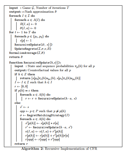
伪代码

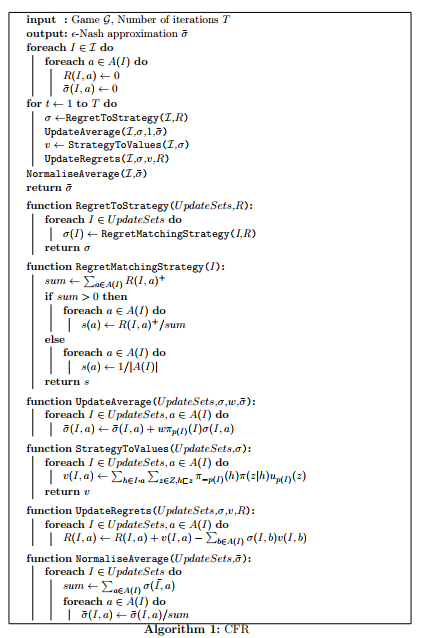
当我们实现CFR算法的时候，可以预先建立博弈问题对应的博弈树，按照深度优先的方式访问博弈树中的节点，从而使得求解算法更加高效

CFR+

MCCFR

posted @ 2022-11-20 18:47 英飞阅读(420) 评论(0) 编辑收藏举报

会员力量，点亮园子希望

刷新页面返回顶部

英飞

卧龙岗闲散人