第七章随笔

第一部分——飞机客户数据分析预测

代码一：读取数据

import pandas as pd
datafile = 'D:/JupyterLab-Portable-3.1.0-3.9/新建文件夹/air_data.csv'
resultfile = 'D:/python123/explore.csv'

data = pd.read_csv(datafile,encoding='utf-8')
explore = data.describe(percentiles=[],include='all').T
explore['null'] = len(data)-explore['count']

explore = explore[['null','max','min']]
explore.columns = [u'空值数',u'非空值数',u'最小值']

'''
这里只选取部分探索结果。
describe()函数自动计算的字段有count（非空值数）、unique（唯一值数）、top（频数最高者）、
freq（最高频数）、mean（平均值）、std（方差）、min（最小值）、50%（中位数）、max（最大值）
'''

explore.to_csv(resultfile)

代码二：分析数据并绘制基本图像

from datetime import datetime

import matplotlib.pyplot as plt

ffp = data['FFP_DATE'].apply(lambda x:datetime.strptime(x,'%Y/%m/%d'))
ffp_year = ffp.map(lambda x : x.year)
fig = plt.figure(figsize=(8,5))
plt.rcParams['font.sans-serif'] = 'SimHei'
plt.rcParams['axes.unicode_minus'] = False
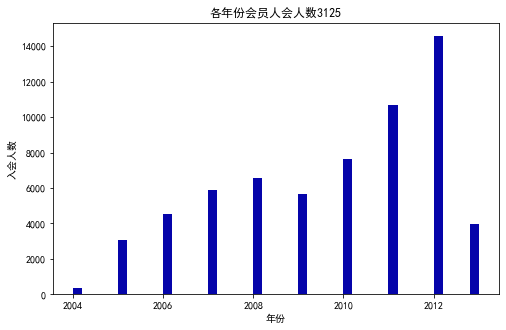
plt.hist(ffp_year,bins='auto',color='#0504aa')
plt.xlabel('年份')
plt.ylabel('入会人数')
plt.title('各年份会员人会人数3125')
plt.show()
plt.close()

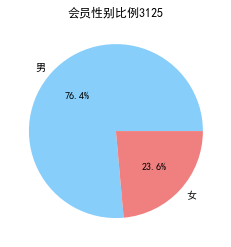
male = pd.value_counts(data['GENDER'])['男']
female = pd.value_counts(data['GENDER'])['女']
fig = plt.figure(figsize=(7,4))
plt.pie([male,female],labels=['男','女'],colors=['lightskyblue','lightcoral'],autopct='%1.1f%%')
plt.title('会员性别比例3125')
plt.show()
plt.close()

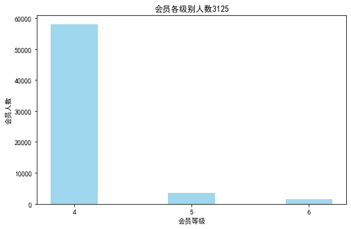
lv_four = pd.value_counts(data['FFP_TIER'])[4]
lv_five = pd.value_counts(data['FFP_TIER'])[5]
lv_six = pd.value_counts(data['FFP_TIER'])[6]
fig = plt.figure(figsize=(8,5))
plt.bar(x=range(3),height=[lv_four,lv_five,lv_six],width=0.4,alpha=0.8,color='skyblue')
plt.xticks([index for index in range(3)],['4','5','6'])
plt.xlabel('会员等级')
plt.ylabel('会员人数')
plt.title('会员各级别人数3125')
plt.show()
plt.close()

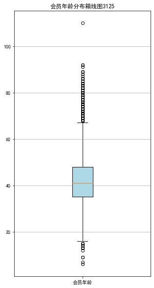
age = data['AGE'].dropna()
age = age.astype('int64')
fig = plt.figure(figsize=(5,10))
plt.boxplot(age,
patch_artist=True,
labels=['会员年龄'],
boxprops={'facecolor':'lightblue'})
plt.title('会员年龄分布箱线图3125')
plt.grid(axis='y')
plt.show()
plt.close()

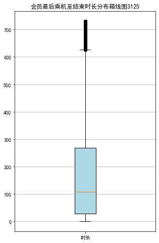
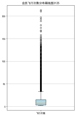
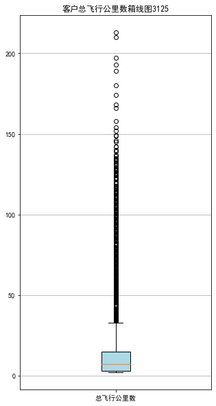
代码三：客户乘机数据分析箱型图

lte = data['LAST_TO_END']
fc = data['FLIGHT_COUNT']
sks = data['SEG_KM_SUM']
fig = plt.figure(figsize=(5,8))
plt.boxplot(lte,
patch_artist=True,
labels=['时长'],
boxprops={'facecolor':'lightblue'})
plt.title('会员最后乘机至结束时长分布箱线图3125')
plt.grid(axis='y')
plt.show()
plt.close()

fig = plt.figure(figsize=(5,8))
plt.boxplot(fc,
patch_artist=True,
labels=['飞行次数'],
boxprops={'facecolor':'lightblue'})
plt.title('会员飞行次数分布箱线图3125')
plt.grid(axis='y')
plt.show()
plt.close()

fig = plt.figure(figsize=(5,10))
plt.boxplot(fc,
patch_artist=True,
labels=['总飞行公里数'],
boxprops={'facecolor':'lightblue'})
plt.title('客户总飞行公里数箱线图3125')
plt.grid(axis='y')
plt.show()
plt.close()

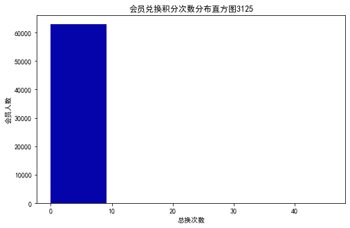
代码四：会员积分数据分析直方图

ec = data['EXCHANGE_COUNT']
fig = plt.figure(figsize=(8,5))
plt.hist(ec,bins=5,color='#0504aa')
plt.xlabel('总换次数')
plt.ylabel('会员人数')
plt.title('会员兑换积分次数分布直方图3125')
plt.show()
plt.close()

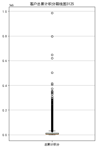
ps = data['Points_Sum']
fig = plt.figure(figsize=(5,8))
plt.boxplot(ps,
patch_artist=True,
labels=['总累计积分'],
boxprops={'facecolor':'lightblue'})
plt.title('客户总累计积分箱线图3125')
plt.grid(axis='y')
plt.show()
plt.close()

 

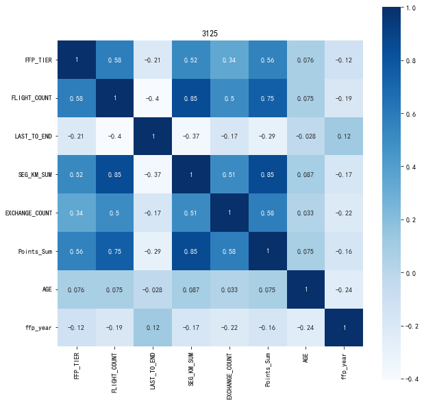
代码五：相关矩阵及热力图

data_corr = data[['FFP_TIER','FLIGHT_COUNT','LAST_TO_END','SEG_KM_SUM','EXCHANGE_COUNT','Points_Sum']]
age1 = data['AGE'].fillna(0)
data_corr['AGE'] = age1.astype('int64')
data_corr['ffp_year'] = ffp_year
dt_corr = data_corr.corr(method='pearson')
print('相关性矩阵为：\n',dt_corr)

import seaborn as sns
plt.subplots(figsize=(10,10))
sns.heatmap(dt_corr,annot=True,vmax=1,square=True,cmap='Blues')
plt.title('3125')
plt.show()
plt.close

相关性矩阵为：
                 FFP_TIER  FLIGHT_COUNT  LAST_TO_END  SEG_KM_SUM  \
FFP_TIER        1.000000      0.582447    -0.206313    0.522350   
FLIGHT_COUNT    0.582447      1.000000    -0.404999    0.850411   
LAST_TO_END    -0.206313     -0.404999     1.000000   -0.369509   
SEG_KM_SUM      0.522350      0.850411    -0.369509    1.000000   
EXCHANGE_COUNT  0.342355      0.502501    -0.169717    0.507819   
Points_Sum      0.559249      0.747092    -0.292027    0.853014   
AGE             0.076245      0.075309    -0.027654    0.087285   
ffp_year       -0.116510     -0.188181     0.117913   -0.171508   

                EXCHANGE_COUNT  Points_Sum       AGE  ffp_year  
FFP_TIER              0.342355    0.559249  0.076245 -0.116510  
FLIGHT_COUNT          0.502501    0.747092  0.075309 -0.188181  
LAST_TO_END          -0.169717   -0.292027 -0.027654  0.117913  
SEG_KM_SUM            0.507819    0.853014  0.087285 -0.171508  
EXCHANGE_COUNT        1.000000    0.578581  0.032760 -0.216610  
Points_Sum            0.578581    1.000000  0.074887 -0.163431  
AGE                   0.032760    0.074887  1.000000 -0.242579  
ffp_year             -0.216610   -0.163431 -0.242579  1.000000  

代码六：进行数据清洗

import numpy as np
cleanedfile = 'D:/python123/data_cleaned.csv'
airline_data = pd.read_csv(datafile,encoding='utf-8')
print('原始数据的形状为：',airline_data.shape)
airline_notnull = airline_data.loc[airline_data['SUM_YR_1'].notnull() &
airline_data['SUM_YR_2'].notnull(),:]
print('删除缺失记录后数据的形状为：',airline_notnull.shape)
index1 = airline_notnull['SUM_YR_1'] != 0
index2 = airline_notnull['SUM_YR_2'] != 0
index3 = (airline_notnull['SEG_KM_SUM'] > 0) & (airline_notnull['avg_discount'] != 0)
index4 = airline_notnull['AGE'] > 100
airline = airline_notnull[(index1 | index2) & index3 & ~index4]
print('数据清洗后数据的形状为：',airline.shape)
airline.to_csv(cleanedfile)

原始数据的形状为： (62988, 44)
删除缺失记录后数据的形状为： (62299, 44)
数据清洗后数据的形状为： (62043, 44)

代码七：

airline = pd.read_csv(cleanedfile,encoding='utf-8')
airline_selection = airline[['FFP_DATE','LOAD_TIME','LAST_TO_END','FLIGHT_COUNT','SEG_KM_SUM','avg_discount']]
print('筛选的属性前5行为：\n',airline_selection.head())

筛选的属性前5行为：
     FFP_DATE  LOAD_TIME  LAST_TO_END  FLIGHT_COUNT  SEG_KM_SUM  avg_discount
0  2006/11/2  2014/3/31            1           210      580717      0.961639
1  2007/2/19  2014/3/31            7           140      293678      1.252314
2   2007/2/1  2014/3/31           11           135      283712      1.254676
3  2008/8/22  2014/3/31           97            23      281336      1.090870
4  2009/4/10  2014/3/31            5           152      309928      0.970658

代码八：

L = pd.to_datetime(airline_selection['LOAD_TIME']) - \
pd.to_datetime(airline_selection['FFP_DATE'])
L = L.astype('str').str.split().str[0]
L = L.astype('int')/30
airline_features = pd.concat([L,airline_selection.iloc[:,2:]],axis=1)
print('构建的LRFMC属性的前5行为：\n',airline_features.head())
from sklearn.preprocessing import StandardScaler
data = StandardScaler().fit_transform(airline_features)
np.savez('D:/python123/airline_scale.npz',data)
print('标准化后LRFMC的5个属性为：\n',data[:5,:])

构建的LRFMC属性的前5行为：
            0  LAST_TO_END  FLIGHT_COUNT  SEG_KM_SUM  avg_discount
0  90.200000            1           210      580717      0.961639
1  86.566667            7           140      293678      1.252314
2  87.166667           11           135      283712      1.254676
3  68.233333           97            23      281336      1.090870
4  60.533333            5           152      309928      0.970658
标准化后LRFMC的5个属性为：
 [[ 1.43579256 -0.94493902 14.03402401 26.76115699  1.29554188]
 [ 1.30723219 -0.91188564  9.07321595 13.12686436  2.86817777]
 [ 1.32846234 -0.88985006  8.71887252 12.65348144  2.88095186]
 [ 0.65853304 -0.41608504  0.78157962 12.54062193  1.99471546]
 [ 0.3860794  -0.92290343  9.92364019 13.89873597  1.34433641]]

代码九：

from sklearn.cluster import KMeans
airline_scale = np.load('D:/python123/airline_scale.npz')['arr_0']
k = 5
kmeans_model = KMeans(n_clusters=k,n_init=4,random_state=123)
fit_kmeans = kmeans_model.fit(airline_scale)
kmeans_cc = kmeans_model.cluster_centers_
print('各类聚类中心为：\n',kmeans_cc)
kmeans_labels = kmeans_model.labels_
print('各样本的类别标签为：\n',kmeans_labels)
r1 = pd.Series(kmeans_model.labels_).value_counts()
print('最终每个类别的数目为：\n',r1)
cluster_center = pd.DataFrame(kmeans_model.cluster_centers_,\
columns=['ZL','ZR','ZF','ZM','ZC'])
cluster_center.index = pd.DataFrame(kmeans_model.labels_).\
drop_duplicates().iloc[:,0]
print(cluster_center)

各类聚类中心为：
 [[ 1.16858148 -0.38005532 -0.08310598 -0.09048484 -0.16482322]
 [-0.70182072 -0.41969421 -0.15465523 -0.15202618 -0.2998482 ]
 [-0.30731409  1.69947472 -0.5752883  -0.53635752 -0.20105777]
 [ 0.48573733 -0.79976463  2.48229556  2.42377224  0.32271572]
 [-0.06479764  0.00270347 -0.269005   -0.28691542  1.907763  ]]
各样本的类别标签为：
 [3 3 3 ... 1 2 2]
最终每个类别的数目为：
 1    23896
0    15534
2    11878
4     5389
3     5346
dtype: int64
         ZL        ZR        ZF        ZM        ZC
0                                                  
3  1.168581 -0.380055 -0.083106 -0.090485 -0.164823
4 -0.701821 -0.419694 -0.154655 -0.152026 -0.299848
0 -0.307314  1.699475 -0.575288 -0.536358 -0.201058
1  0.485737 -0.799765  2.482296  2.423772  0.322716
2 -0.064798  0.002703 -0.269005 -0.286915  1.907763

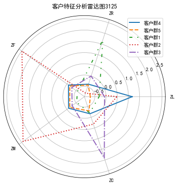
代码十：绘制客户分群雷达图

%matplotlib inline
labels = ['ZL','ZR','ZF','ZM','ZC']
legen = ['客户群' + str(i + 1) for i in cluster_center.index]
lstype = ['-','--',(0,(3,5,1,5,1,5)),':','-.']
kinds = list(cluster_center.iloc[:,0])
cluster_center = pd.concat([cluster_center,cluster_center[['ZL']]],axis=1)
centers = np.array(cluster_center.iloc[:,0:])

n = len(labels)
angle = np.linspace(0,2 * np.pi,n,endpoint=False)
angle = np.concatenate((angle,[angle[0]]))

fig = plt.figure(figsize=(8,6))
ax = fig.add_subplot(111,polar=True)
for i in range(len(kinds)):
ax.plot(angle,centers[i],linestyle=lstype[i],linewidth=2,label=kinds[i])
ax.set_thetagrids(angle[:-1] * 180 / np.pi,labels)
plt.title('客户特征分析雷达图3125')
plt.legend(legen)
plt.show()
plt.close()

第二部分：电信客户流失分析预测

 代码1：读取并简单分析数据

plt.rc("font",family="SimHei",size="12") #解决中文无法显示的问题
data = pd.read_csv('D:/JupyterLab-Portable-3.1.0-3.9/新建文件夹/WA_Fn-UseC_-Telco-Customer-Churn.csv') # 导入数据
data.shape # 查看数据大小

(7043, 21)

data.head()

 

customerID	gender	SeniorCitizen	Partner	Dependents	tenure	PhoneService	MultipleLines	InternetService	OnlineSecurity	...	DeviceProtection	TechSupport	StreamingTV	StreamingMovies	Contract	PaperlessBilling	PaymentMethod	MonthlyCharges	TotalCharges	Churn
0	7590-VHVEG	Female	0	Yes	No	1	No	No phone service	DSL	No	...	No	No	No	No	Month-to-month	Yes	Electronic check	29.85	29.85	No
1	5575-GNVDE	Male	0	No	No	34	Yes	No	DSL	Yes	...	Yes	No	No	No	One year	No	Mailed check	56.95	1889.5	No
2	3668-QPYBK	Male	0	No	No	2	Yes	No	DSL	Yes	...	No	No	No	No	Month-to-month	Yes	Mailed check	53.85	108.15	Yes
3	7795-CFOCW	Male	0	No	No	45	No	No phone service	DSL	Yes	...	Yes	Yes	No	No	One year	No	Bank transfer (automatic)	42.30	1840.75	No
4	9237-HQITU	Female	0	No	No	2	Yes	No	Fiber optic	No	...	No	No	No	No	Month-to-month	Yes	Electronic check	70.70	151.65	Yes

5 rows × 21 columns

data.describe()  #描述性统计信息

	SeniorCitizen	tenure	MonthlyCharges
count	7043.000000	7043.000000	7043.000000
mean	0.162147	32.371149	64.761692
std	0.368612	24.559481	30.090047
min	0.000000	0.000000	18.250000
25%	0.000000	9.000000	35.500000
50%	0.000000	29.000000	70.350000
75%	0.000000	55.000000	89.850000
max	1.000000	72.000000	118.750000

代码2：客户流失数据分析

data['Churn'].value_counts()  #查找缺失值

No     5174
Yes    1869
Name: Churn, dtype: int64

#数据集中有5174名用户没流失，有1869名客户流失，数据集不均衡。

data.dtypes  #查看数据类型

customerID           object
gender               object
SeniorCitizen         int64
Partner              object
Dependents           object
tenure                int64
PhoneService         object
MultipleLines        object
InternetService      object
OnlineSecurity       object
OnlineBackup         object
DeviceProtection     object
TechSupport          object
StreamingTV          object
StreamingMovies      object
Contract             object
PaperlessBilling     object
PaymentMethod        object
MonthlyCharges      float64
TotalCharges         object
Churn                object
dtype: object

#TotalCharges表示总费用，这里为对象类型，需要转换为float类型
data['TotalCharges']=data['TotalCharges'].apply(pd.to_numeric, errors="ignore")
data['TotalCharges'].describe()

count     7043
unique    6531
top           
freq        11
Name: TotalCharges, dtype: object

#数据归一化处理
#对Churn列中的YES和No分别用1和0替换，方便后续处理
data['Churn'].replace(to_replace='Yes',value=1,inplace=True)
data['Churn'].replace(to_replace='No',value=0,inplace=True)
data['Churn'].describe()

count    7043.000000
mean        0.265370
std         0.441561
min         0.000000
25%         0.000000
50%         0.000000
75%         1.000000
max         1.000000
Name: Churn, dtype: float64

data.info()  #数据预览

<class 'pandas.core.frame.DataFrame'>
RangeIndex: 7043 entries, 0 to 7042
Data columns (total 21 columns):
 #   Column            Non-Null Count  Dtype  
---  ------            --------------  -----  
 0   customerID        7043 non-null   object 
 1   gender            7043 non-null   object 
 2   SeniorCitizen     7043 non-null   int64  
 3   Partner           7043 non-null   object 
 4   Dependents        7043 non-null   object 
 5   tenure            7043 non-null   int64  
 6   PhoneService      7043 non-null   object 
 7   MultipleLines     7043 non-null   object 
 8   InternetService   7043 non-null   object 
 9   OnlineSecurity    7043 non-null   object 
 10  OnlineBackup      7043 non-null   object 
 11  DeviceProtection  7043 non-null   object 
 12  TechSupport       7043 non-null   object 
 13  StreamingTV       7043 non-null   object 
 14  StreamingMovies   7043 non-null   object 
 15  Contract          7043 non-null   object 
 16  PaperlessBilling  7043 non-null   object 
 17  PaymentMethod     7043 non-null   object 
 18  MonthlyCharges    7043 non-null   float64
 19  TotalCharges      7043 non-null   object 
 20  Churn             7043 non-null   int64  
dtypes: float64(1), int64(3), object(17)
memory usage: 1.1+ MB

#在数据预览过后，我们发现不存在缺失值，并且许多特征维度的数据类型均为python默认的object对象类型。

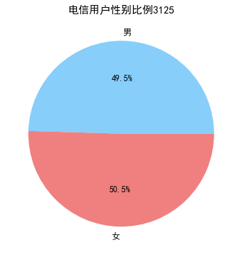
 代码3：绘制电信客户性别饼图和绘制客户流失情况饼图

plt.rcParams['font.sans-serif']='SimHei'
plt.rcParams['axes.unicode_minus']='False'
#提取会员不同性别人数
male=pd.value_counts(data['gender'])['Female']
female=pd.value_counts(data['gender'])['Male']
#绘制会员性别比例饼图
fig=plt.figure(figsize=(10,6))
plt.pie([male,female],labels=['男','女'],colors=['lightskyblue','lightcoral'],autopct='%1.1f%%')
plt.title('电信用户性别比例3125',fontsize=15)
plt.show()
plt.close()

churnvalue=data[ "Churn" ].value_counts()
labels=data["Churn"].value_counts().index

plt.figure(figsize=(6,6))
plt.pie(churnvalue,labels=labels,colors=["blue","yellow"],explode=(0.1,0),autopct='%1.1f', shadow=True)
plt.title('客户流失情况饼图3125',fontsize=15)
plt.show()

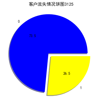
#由图中结果可以看出，流失客户占整体客户的26.5%。

代码4：客户流失影响直方图

#性别、老年人、配偶、亲属对流客户流失率的影响
plt.figure(figsize=(10,10))
plt.subplot(2,2,1)
gender=sns.countplot(x='gender',hue='Churn',data=data,palette='Set2') #palette参数表示设置颜色，设置为主颜色paste12
plt.xlabel('性别')
plt.title('不同性别客户流失直方图3125',fontsize=15)

plt.subplot(2,2,2)
seniorcitizen=sns.countplot(x='SeniorCitizen',hue='Churn',data=data,palette='Set2')
plt.xlabel('老年人')
plt.title('老年人客户流失直方图3125',fontsize=15)

plt.subplot(2,2,3)
partner=sns.countplot(x='Partner',hue='Churn',data=data,palette='Set2')
plt.xlabel('配偶')
plt.title('是否有配偶客户流失直方图3125',fontsize=15)

plt.subplot(2,2,4)
dependents=sns.countplot(x='Dependents',hue='Churn',data=data,palette='Set2')
plt.xlabel('亲属')
plt.title('亲属客户流失直方图3125',fontsize=15)
plt.show()

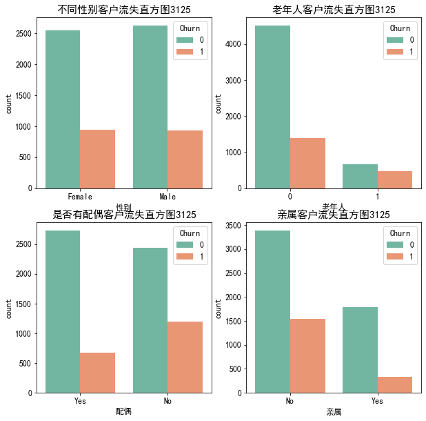
#可以看出，男性与女性用户之间的流失情况基本没有差异，而在老年用户中流失占比明显比非老年用户更高，
 在所有数据中未婚与已婚人数基本持平，但未婚中流失人数比已婚中的流失人数高出了快一倍，
 从经济独立情况来看，经济未独立的用户流失率要远远高于经济独立的用户。

代码5：特征值

#提取特征
charges=data.iloc[:,1:20]
#对特征进行编码
corrdf=charges.apply(lambda x:pd.factorize(x)[0])
corrdf.head()

gender	SeniorCitizen	Partner	Dependents	tenure	PhoneService	MultipleLines	InternetService	OnlineSecurity	OnlineBackup	DeviceProtection	TechSupport	StreamingTV	StreamingMovies	Contract	PaperlessBilling	PaymentMethod	MonthlyCharges	TotalCharges
0	0	0	0	0	0	0	0	0	0	0	0	0	0	0	0	0	0	0	0
1	1	0	1	0	1	1	1	0	1	1	1	0	0	0	1	1	1	1	1
2	1	0	1	0	2	1	1	0	1	0	0	0	0	0	0	0	1	2	2
3	1	0	1	0	3	0	0	0	1	1	1	1	0	0	1	1	2	3	3
4	0	0	1	0	2	1	1	1	0	1	0	0	0	0	0	0	0	4	4

 

#构建相关矩阵
corr = corrdf.corr()
corr

	gender	SeniorCitizen	Partner	Dependents	tenure	PhoneService	MultipleLines	InternetService	OnlineSecurity	OnlineBackup	DeviceProtection	TechSupport	StreamingTV	StreamingMovies	Contract	PaperlessBilling	PaymentMethod	MonthlyCharges	TotalCharges
gender	1.000000	-0.001874	0.001808	0.010517	-0.000013	-0.006488	-0.009451	-0.000863	-0.003429	0.012230	0.005092	0.000985	0.001156	-0.000191	0.000126	0.011754	-0.005209	-0.008072	-0.012302
SeniorCitizen	-0.001874	1.000000	-0.016479	-0.211185	0.010834	0.008576	0.113791	-0.032310	-0.210897	-0.144828	-0.157095	-0.223770	-0.130130	-0.120802	-0.142554	-0.156530	-0.093704	0.049649	0.023880
Partner	0.001808	-0.016479	1.000000	-0.452676	-0.101985	-0.017706	-0.117307	-0.000891	-0.081850	0.090753	-0.094451	-0.069072	-0.080127	-0.075779	-0.294806	-0.014877	-0.133115	-0.036054	-0.042628
Dependents	0.010517	-0.211185	-0.452676	1.000000	0.048514	-0.001762	-0.019657	0.044590	0.190523	0.062775	0.156439	0.180832	0.140395	0.125820	0.243187	0.111377	0.123844	-0.029390	0.006300
tenure	-0.000013	0.010834	-0.101985	0.048514	1.000000	-0.018799	0.063510	-0.012008	0.017083	-0.064613	0.037174	0.033108	0.027090	0.031491	0.122446	-0.011129	0.075379	0.041647	0.108142
PhoneService	-0.006488	0.008576	-0.017706	-0.001762	-0.018799	1.000000	0.675070	0.387436	0.125353	0.129770	0.138755	0.123350	0.171538	0.165205	0.002247	-0.016505	-0.004070	-0.141829	-0.029806
MultipleLines	-0.009451	0.113791	-0.117307	-0.019657	0.063510	0.675070	1.000000	0.186826	-0.066844	-0.130619	-0.013069	-0.066684	0.030195	0.028187	0.083343	-0.133255	0.025676	0.024338	0.015373
InternetService	-0.000863	-0.032310	-0.000891	0.044590	-0.012008	0.387436	0.186826	1.000000	0.607788	0.650962	0.662957	0.609795	0.712890	0.709020	0.099721	0.138625	0.008124	-0.289963	-0.038247
OnlineSecurity	-0.003429	-0.210897	-0.081850	0.190523	0.017083	0.125353	-0.066844	0.607788	1.000000	0.621739	0.749040	0.791225	0.701976	0.704984	0.389978	0.334003	0.213800	-0.220566	-0.026788
OnlineBackup	0.012230	-0.144828	0.090753	0.062775	-0.064613	0.129770	-0.130619	0.650962	0.621739	1.000000	0.601503	0.617003	0.604117	0.606863	0.035407	0.260715	0.003183	-0.284344	-0.054537
DeviceProtection	0.005092	-0.157095	-0.094451	0.156439	0.037174	0.138755	-0.013069	0.662957	0.749040	0.601503	1.000000	0.767970	0.763279	0.766821	0.390216	0.276326	0.191746	-0.220217	-0.025159
TechSupport	0.000985	-0.223770	-0.069072	0.180832	0.033108	0.123350	-0.066684	0.609795	0.791225	0.617003	0.767970	1.000000	0.737578	0.737123	0.418440	0.310749	0.216878	-0.213417	-0.021945
StreamingTV	0.001156	-0.130130	-0.080127	0.140395	0.027090	0.171538	0.030195	0.712890	0.701976	0.604117	0.763279	0.737578	1.000000	0.809608	0.327951	0.203907	0.117618	-0.230706	-0.018643
StreamingMovies	-0.000191	-0.120802	-0.075779	0.125820	0.031491	0.165205	0.028187	0.709020	0.704984	0.606863	0.766821	0.737123	0.809608	1.000000	0.330993	0.211818	0.123869	-0.241007	-0.026122
Contract	0.000126	-0.142554	-0.294806	0.243187	0.122446	0.002247	0.083343	0.099721	0.389978	0.035407	0.390216	0.418440	0.327951	0.330993	1.000000	0.176733	0.358913	-0.007618	0.051905
PaperlessBilling	0.011754	-0.156530	-0.014877	0.111377	-0.011129	-0.016505	-0.133255	0.138625	0.334003	0.260715	0.276326	0.310749	0.203907	0.211818	0.176733	1.000000	0.101480	-0.087229	-0.011179
PaymentMethod	-0.005209	-0.093704	-0.133115	0.123844	0.075379	-0.004070	0.025676	0.008124	0.213800	0.003183	0.191746	0.216878	0.117618	0.123869	0.358913	0.101480	1.000000	-0.009290	0.008458
MonthlyCharges	-0.008072	0.049649	-0.036054	-0.029390	0.041647	-0.141829	0.024338	-0.289963	-0.220566	-0.284344	-0.220217	-0.213417	-0.230706	-0.241007	-0.007618	-0.087229	-0.009290	1.000000	0.267898
TotalCharges	-0.012302	0.023880	-0.042628	0.006300	0.108142	-0.029806	0.015373	-0.038247	-0.026788	-0.054537	-0.025159	-0.021945	-0.018643	-0.026122	0.051905	-0.011179	0.008458	0.267898	1.000000

代码6：热力图

'''
heatmap 使用热力图展示系数矩阵情况
linewidths 热力图矩阵之间的间隔大小
annot 设定是否显示每个色块系数值
'''
plt.figure(figsize=(30,20))
ax=sns.heatmap(corr,xticklabels=corr.columns,yticklabels=corr.columns,linewidths=0.2,cmap='YlGnBu',annot=True)
plt.title('相关系数热力图3125',fontsize=15)
plt.show()

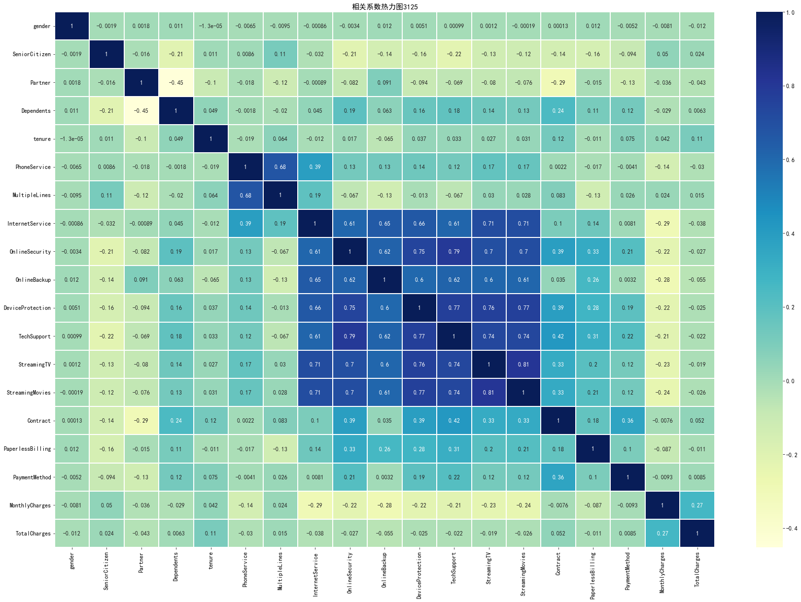
#从上图可以看出，互联网服务、网络安全服务、在线备份业务、设备保护业务、技术支持服务、网络电视和网络电影之间存在较强的相关性，
#多线业务和电话服务之间也有很强的相关性，并且都呈强正相关关系。

代码7：电信用户是否流失与各变量之间的相关性

tel_dummies=pd.get_dummies(data.iloc[:,1:21])
tel_dummies.head()

plt.figure(figsize=(15,8))
tel_dummies.corr()['Churn'].sort_values(ascending=False).plot(kind='bar')
plt.title('电信用户是否流失与各变量之间的相关性图3125',fontsize=15)
plt.show()

 

 

 

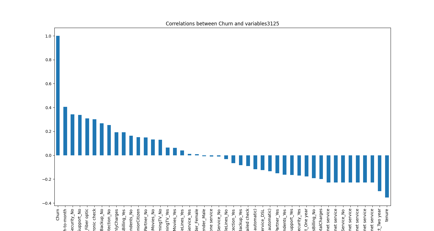
#由图上可以看出，变量gender 和 PhoneService 处于图形中间，其值接近于 0 ，这两个变量对电信客户流失预测影响非常小，可以直接舍弃。

代码8：网络安全服务、在线备份业务、设备保护业务、技术支持服务、网络电视、网络电影和无互联网服务对客户流失率的影响

#网络安全服务、在线备份业务、设备保护业务、技术支持服务、网络电视、网络电影和无互联网服务对客户流失率的影响
covariable=['OnlineSecurity','OnlineBackup','DeviceProtection','TechSupport','StreamingTV','StreamingMovies']
plt.figure(figsize=(17,10))
for i,item in enumerate(covariable):
plt.subplot(2,3,(i+1))
ax=sns.countplot(x=item,hue='Churn',data=data,palette='Set2',order=['Yes','No','No internet service'])
plt.xlabel(str(item))
plt.title(str(item)+'对客户流失的影响3125',fontsize=15)
i=i+1
plt.show()

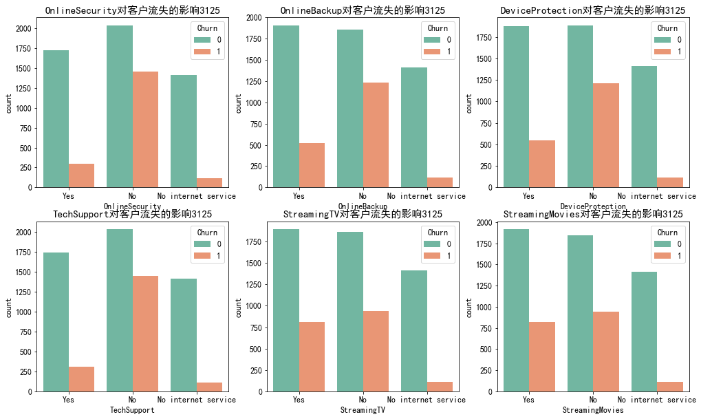
#由上图可以看出，在网络安全服务、在线备份业务、设备保护业务、技术支持服务、网络电视和网络电影六个变量中，没有互联网服务的客户流失率值是相同的，都是相对较低。
#这可能是因为以上六个因素只有在客户使用互联网服务时才会影响客户的决策，这六个因素不会对不使用互联网服务的客户决定是否流失产生推论效应。

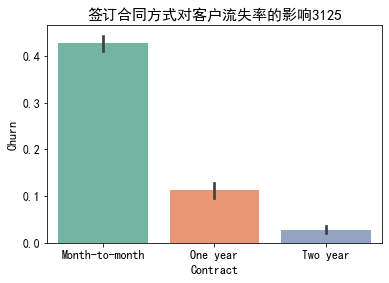
代码9：绘制签订合同方式对客户流失率的影响直方图和绘制付款方式对客户流失率的影响直方图

#签订合同方式对客户流失率的影响
ax=sns.barplot(x='Contract',y='Churn',data=data,palette='Set2',order=['Month-to-month','One year','Two year'])
plt.title('签订合同方式对客户流失率的影响3125',fontsize=15)
plt.show()

#由图可以看出，签订合同方式对客户流失率影响为：按月签订 > 按一年签订 > 按两年签订，这可能表明，设定长期合同对留住现有客户更有效。

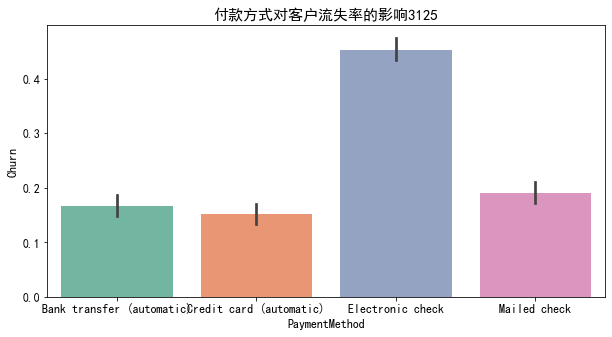
#付款方式对客户流失率的影响
plt.figure(figsize=(10,5))
ax=sns.barplot(x='PaymentMethod',y='Churn',data=data,palette='Set2',
order=['Bank transfer (automatic)','Credit card (automatic)','Electronic check','Mailed check'])
plt.title('付款方式对客户流失率的影响3125',fontsize=15)
plt.show()

#由图可以看出，在四种支付方式中，使用Electronic check的用户流流失率最高，其他三种支付方式基本持平，因此可以推断电子账单在设计上影响用户体验。

通过上述分析，我们可以大致勾勒出容易流失的用户特征：

老年用户与未婚且经济未独立的青少年用户更容易流失。

电话服务对用户的流失没有直接的影响。

提供的各项网络服务项目能够降低用户的流失率。

签订合同越久，用户的留存率越高。

采用electronic check支付的用户更易流失。

针对上述诊断结果，可有针对性的对此提出建议：
推荐老年用户与青少年用户采用数字网络，且签订2年期合同（可以各种辅助优惠等营销手段来提高2年期合同的签订率），
若能开通相关网络服务可增加用户粘性，因此可增加这块业务的推广，同时考虑改善电子账单支付的用户体验。