

使用LSTM进行时间序列预测PyTorch版本
前言
- 24小时气温数据,
- 一个月的产品价格数据,
- 某一公司股票价格年度数据。
- 。。。。。。
高级深度学习模型,比如长短期记忆网络(LSTM),能够捕获到时间序列数据中的变化模式,进而能够预测数据的未来趋势。本文中,我们将使用pytorch这个深度学习库,来实现利用LSTM算法对时间序列数据进行预测。
在开始讲述之前,我们先导入必要的库,
import torch
import torch.nn as nn

import seaborn as sns
import numpy as np
import pandas as pd
import matplotlib.pyplot as plt

%matplotlib inline
数据集
我们将使用Seaborn库的内建数据集。让我们打印一下Seaborn的所有内建数据库:
sns.get_dataset_names()
输出结果为:
['anagrams',
 'anscombe',
 'attention',
 'brain_networks',
 'car_crashes',
 'diamonds',
 'dots',
 'dowjones',
 'exercise',
 'flights',
 'fmri',
 'geyser',
 'glue',
 'healthexp',
 'iris',
 'mpg',
 'penguins',
 'planets',
 'seaice',
 'taxis',
 'tips',
 'titanic']
我们将使用flights数据集。可以用如下代码导入:
flight_data = sns.load_dataset("flights")
flight_data.head()
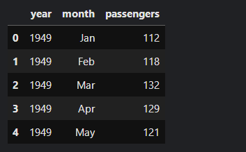
数据集有3列:年,月和乘客数量。乘客数量一列描述了单月内航班乘客总数。
数据集的形状:
flight_data.shape
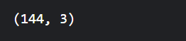
可以看到,一共有144行和3列数据,即数据集包含12年的乘客记录。 我们的任务是利用前132个月的数据预测最后12个月乘客数。也就是说前132个月的数据用作训练,最后12个月的数据用作验证以评估模型。
让我们来绘制每个月乘客出行的频率,
fig_size = plt.rcParams["figure.figsize"]
fig_size[0] = 15
fig_size[1] = 5
plt.rcParams["figure.figsize"] = fig_size

plt.title('Month vs Passenger')
plt.ylabel('Total Passengers')
plt.xlabel('Months')
plt.grid(True)
plt.autoscale(axis='x',tight=True)
plt.plot(flight_data['passengers'])
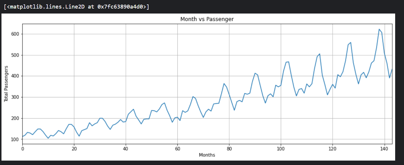
如图所示,多年来,乘飞机旅行的平均人数增加了。一年内旅行的乘客数量是波动的,这是有道理的,因为在夏季或冬季休假期间,旅行的乘客数量比一年中的其他时间增加。
构建LSTM需要的样本集
我们先看一下数据列中数据的类型,
flight_data.info()
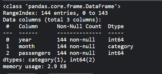
- 数据处理的第一步是将乘客数量一列的数据类型转换为
float,
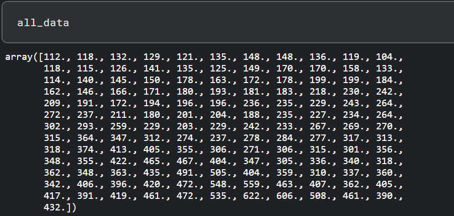
all_data = flight_data['passengers'].values.astype(float)
现在,如果你打印all_data这个numpy数组,你应该看到以下float类型的值。
- 接下来,我们将把我们的数据集分为训练集和测试集。LSTM算法将在训练集上进行训练。然后,该模型将被用来对测试集进行预测。预测结果将与测试集的实际值进行比较,以评估训练模型的性能。前132条记录将被用来训练模型,最后12条记录将被用作测试集。下面的代码将数据分为训练集和测试集。
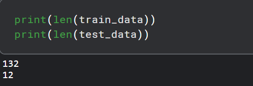
test_data_size = 12

train_data = all_data[:-test_data_size]
test_data = all_data[-test_data_size:]
让我们打印一下训练集和测试集的样本个数:
- 我们的数据集目前还没有被归一化(normalization)。最初几年的乘客总数与后来几年的乘客总数相比要少得多。对于时间序列预测来说,将数据归一化是非常重要的。我们将对数据集进行最小/最大缩放,使数据在一定的最小值和最大值范围内归一化。我们将使用sklearn.preprocessing模块中的MinMaxScaler类来缩放我们的数据。下面的代码使用最小/最大缩放器对我们的数据进行归一化处理,最小值和最大值分别为-1和1。
from sklearn.preprocessing import MinMaxScaler

scaler = MinMaxScaler(feature_range=(-1, 1))
train_data_normalized = scaler.fit_transform(train_data .reshape(-1, 1))
让我们打印出经过归一化处理之后的前5条和最后5条数据,
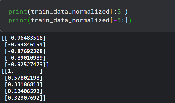
这里需要提到的是,数据归一化只适用于训练数据,而不是测试数据。如果在测试数据上应用归一化,有可能会有一些信息从训练集泄露到测试集。
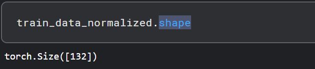
- 下一步是将我们的数据集转换成张量,因为PyTorch模型是使用张量进行训练的。为了将数据集转换为张量,我们可以简单地将我们的数据集传递给FloatTensor对象的构造函数,如下所示。
train_data_normalized = torch.FloatTensor(train_data_normalized).view(-1)
- 最后的预处理步骤是将我们的训练数据转换成序列和相应的标签。你可以使用任何序列长度,这取决于领域知识。然而,在我们的数据集中,使用12的序列长度是很方便的,因为我们有月度数据,一年有12个月。如果我们有每日数据,更好的序列长度是365,即一年中的天数。因此,我们将训练时的输入序列长度设置为12。
train_window = 12
def create_inout_sequences(input_data, tw):
    inout_seq = []
    L = len(input_data)
    for i in range(L-tw):
        train_seq = input_data[i:i+tw]
        train_label = input_data[i+tw:i+tw+1]
        inout_seq.append((train_seq ,train_label))
    return inout_seq
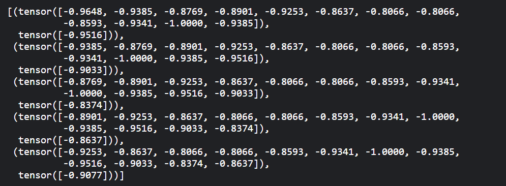
运行下面的代码来创造用来训练的序列和对应的标签:
train_inout_seq = create_inout_sequences(train_data_normalized, train_window)
train_inout_seq[:5]
创建LSTM模型
我们已经预处理了数据,现在是时候训练我们的模型了。我们将定义一个LSTM类,它继承于PyTorch库的nn.Module类。
class LSTM(nn.Module):
    def __init__(self,input_size=1,hidden_layer_size=100,output_size=1):
        super().__init__()
        self.hidden_layer_size = hidden_layer_size
        self.lstm = nn.LSTM(input_size,hidden_layer_size)
        self.linear = nn.Linear(hidden_layer_size,output_size)
        self.hidden_cell = (torch.zeros(1,1,self.hidden_layer_size),torch.zeros(1,1,self.hidden_layer_size))

    def forward(self,input_seq):
        lstm_out,self.hidden_cell = self.lstm(input_seq.view(len(input_seq),1,-1), self.hidden_cell)
        //predictions.shape:[L,1]
        predictions = self.linear(lstm_out.view(len(input_seq), -1))
       //predictions[-1].shape:[1]
        return predictions[-1]
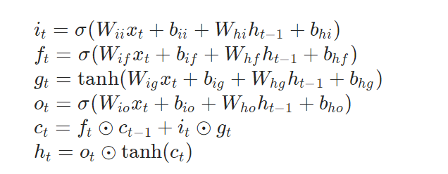
对于pytorch里面的LSTM类,我们可以查阅一下官方文档,来看一下它的用法,
CLASS torch.nn.LSTM(*args, **kwargs)
Applies a multi-layer long short-term memory (LSTM) RNN to an input sequence。For each element in the input sequence, each layer computes the following function:
Parameters:
-
input_size – The number of expected features in the input x
-
hidden_size – The number of features in the hidden state h
-
num_layers – Number of recurrent layers. E.g., setting
num_layers=2would mean stacking two LSTMs together to form a stacked LSTM, with the second LSTM taking in outputs of the first LSTM and computing the final results. Default: 1 -
bias – If
False, then the layer does not use bias weights b_ih and b_hh. Default:True -
batch_first – If
True, then the input and output tensors are provided as (batch, seq, feature) instead of (seq, batch, feature). Note that this does not apply to hidden or cell states. See the Inputs/Outputs sections below for details. Default: False -
dropout – If non-zero, introduces a Dropout layer on the outputs of each LSTM layer except the last layer, with dropout probability equal to
dropout. Default: 0 -
bidirectional – If
True, becomes a bidirectional LSTM. Default:False -
proj_size – If
> 0, will use LSTM with projections of corresponding size. Default: 0
Inputs: input, (h_0, c_0)
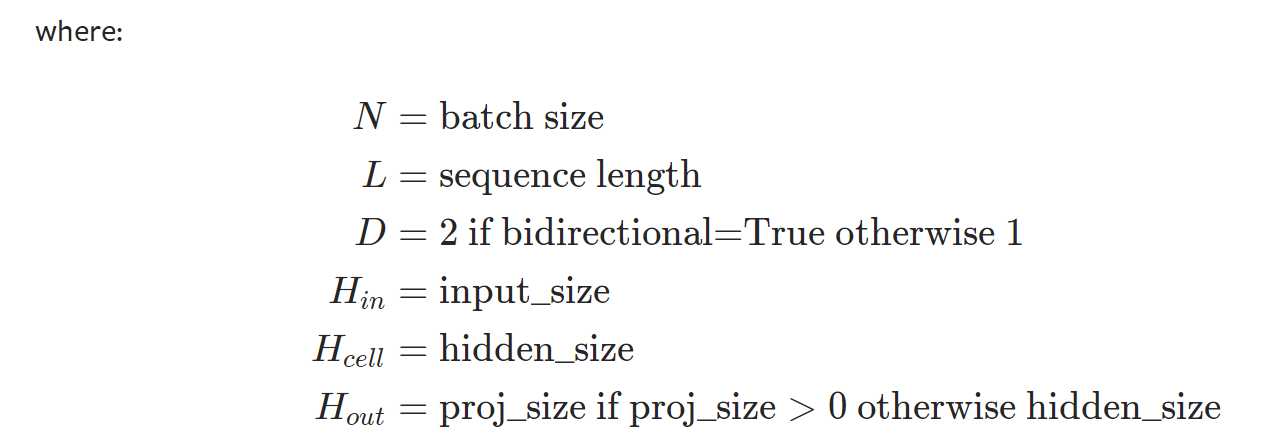
- input: tensor of shape $(L, H_{in}) $for unbatched input, $(L, N, H_{in})$when batch_first=False or $(N, L, H_{in})$when batch_first=True containing the features of the input sequence. The input can also be a packed variable length sequence. See torch.nn.utils.rnn.pack_padded_sequence() or torch.nn.utils.rnn.pack_sequence() for details.
- h_0: tensor of shape $(D * \text{num_layers}, H_{out})$ for unbatched input or $(D * \text{num_layers}, N, H_{out})$ containing the initial hidden state(LSTM隐藏状态$h_t$的初始值) for each element in the input sequence. Defaults to zeros if $(h_0, c_0)$ is not provided.
- c_0: tensor of shape $(D * \text{num_layers}, H_{cell})$ for unbatched input or $(D * \text{num_layers}, N, H_{cell})$ containing the initial cell state(LSTM内部状态$c_t$的初始值) for each element in the input sequence. Defaults to zeros if (h_0, c_0) is not provided.
Outputs: output, (h_n, c_n)
- output: tensor of shape $(L, D * H_{out})$for unbatched input, $(L, N, D * H_{out})$when batch_first=False or $(N, L, D * H_{out})$ when batch_first=True containing the output features (h_t) from the last layer of the LSTM, for each t. If a torch.nn.utils.rnn.PackedSequence has been given as the input, the output will also be a packed sequence. When bidirectional=True, output will contain a concatenation of the forward and reverse hidden states at each time step in the sequence.
- h_n: tensor of shape $(D * \text{num_layers}, H_{out})$ for unbatched input or $(D * \text{num_layers}, N, H_{out})$ containing the final hidden state for each element in the sequence. When bidirectional=True, h_n will contain a concatenation of the final forward and reverse hidden states, respectively.
- c_n: tensor of shape $(D * \text{num_layers}, H_{cell})$ for unbatched input or $(D * \text{num_layers}, N, H_{cell})$ containing the final cell state for each element in the sequence. When bidirectional=True, c_n will contain a concatenation of the final forward and reverse cell states, respectively.
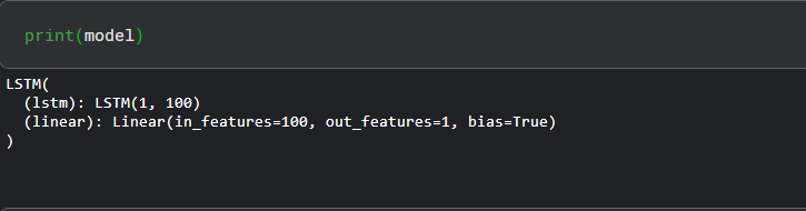
model = LSTM()
loss_function = nn.MSELoss()
optimizer = torch.optim.Adam(model.parameters(), lr=0.001)
下面让我们打印一下这个模型,
训练模型和预测
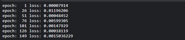
我们将对我们的模型进行150次的训练。如果你愿意,你可以尝试更多次。损失将在每25次后被打印出来。
epochs = 150

for i in range(epochs):
    for seq, labels in train_inout_seq:
        optimizer.zero_grad()
        model.hidden_cell = (torch.zeros(1, 1, model.hidden_layer_size),
                        torch.zeros(1, 1, model.hidden_layer_size))

        y_pred = model(seq)

        single_loss = loss_function(y_pred, labels)
        single_loss.backward()
        optimizer.step()

    if i%25 == 1:
        print(f'epoch: {i:3} loss: {single_loss.item():10.8f}')

print(f'epoch: {i:3} loss: {single_loss.item():10.10f}')
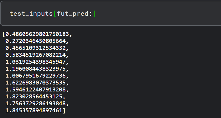
现在我们的模型已经训练完毕,我们可以开始进行预测。由于我们的测试集包含了过去12个月的乘客数据,而我们的模型被训练为使用12的序列长度进行预测。我们将首先从训练集中筛选出最后12个值。
fut_pred = 12

test_inputs = train_data_normalized[-train_window:].tolist()
print(test_inputs)

model.eval()

for i in range(fut_pred):
    seq = torch.FloatTensor(test_inputs[-train_window:])
    with torch.no_grad():
        model.hidden = (torch.zeros(1, 1, model.hidden_layer_size),
                        torch.zeros(1, 1, model.hidden_layer_size))
        test_inputs.append(model(seq).item())
如果你打印test_inputs列表的长度,你会发现它包含24个item。最后12个预测项可以打印出来,如下所示:
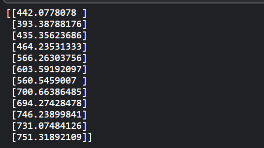
由于我们对训练的数据集进行了归一化处理,预测值也被归一化了。我们需要将归一化的预测值转换成实际的预测值。我们可以通过将归一化的值传递给min/max scaler对象的inverse_transform方法来实现,
actual_predictions = scaler.inverse_transform(np.array(test_inputs[train_window:] ).reshape(-1, 1))
print(actual_predictions)
现在让我们把预测值与实际值作对比。请看下面的代码。
x = np.arange(132, 144, 1)
print(x)
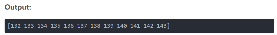
在上面的脚本中,我们创建了一个包含过去12个月的数值的列表。第一个月的索引值为0,因此最后一个月的索引值为143。
在下面的脚本中,我们将绘制144个月的乘客总数,以及过去12个月的预测乘客数。
plt.title('Month vs Passenger')
plt.ylabel('Total Passengers')
plt.grid(True)
plt.autoscale(axis='x', tight=True)
plt.plot(flight_data['passengers'])
plt.plot(x,actual_predictions)
plt.show()
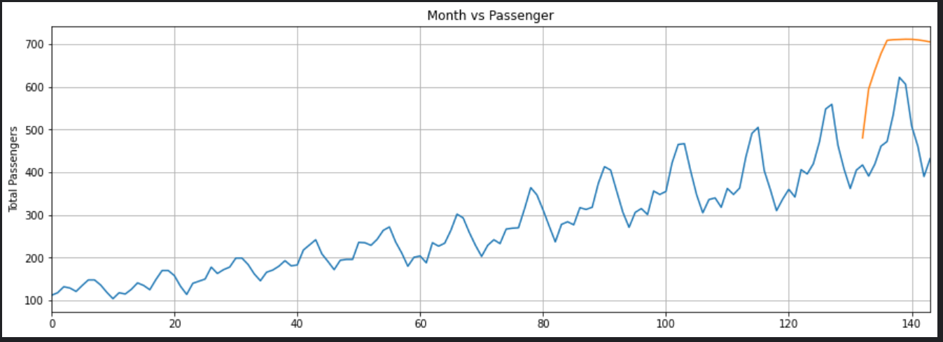
我们的LSTM所做的预测是由橙色的线条描述的。你可以看到,我们的算法不是太准确,但它仍然能够捕捉到过去12个月内旅行的乘客总数的上升趋势,以及偶尔的波动。你可以尝试在LSTM层中使用更多的epochs和更多的神经元,看看你是否能获得更好的性能。
为了更好地了解输出,我们可以绘制过去12个月的实际和预测的乘客数量,如下所示:
plt.title('Month vs Passenger')
plt.ylabel('Total Passengers')
plt.grid(True)
plt.autoscale(axis='x', tight=True)

plt.plot(flight_data['passengers'][-train_window:])
plt.plot(x,actual_predictions)
plt.show()
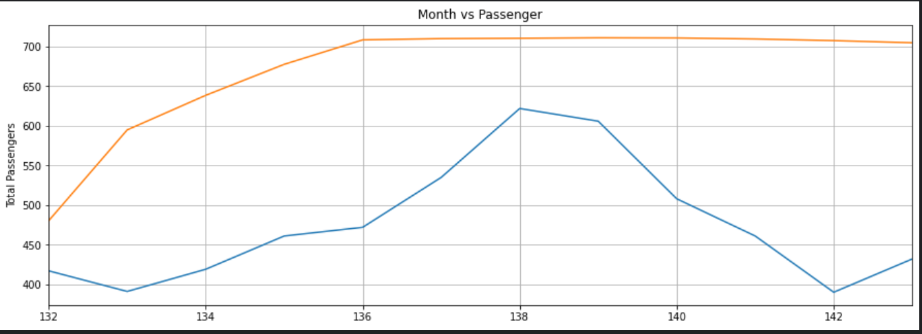
同样,预测不是很准确,但该算法能够捕捉到未来几个月的乘客数量应该高于前几个月的趋势,偶尔会有波动。
