BiLSTM+CRF及pytorch实现

目录

• 前言
• BiLSTM+CRF模型
  • 概述
  • 为什么需要添加CRF层？
  • CRF层
    • Emission score
    • Transition score
  • CRF损失函数
    • 实际路径得分
    • 所有可能的路径的总得分
  • 为新的句子推断标签(维特比解码)
• pytorch实现
• 参考

前言

对于命名实体识别任务，基于神经网络的方法非常普遍。例如，Neural Architectures for Named Entity Recognition提出了一个使用word and character embeddings的BiLSTM-CRF命名实体识别模型。我将以本文中的模型为例来解释CRF层是如何工作的。如果你不知道BiLSTM和CRF的细节，请记住它们是命名实体识别模型中的两个不同的层。

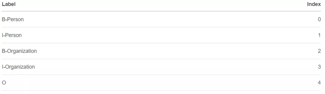
在开始我们下面将进行的讨论之前，我们先假设，我们有一个数据集，其中有两个实体类型：Person和Organization。但是，事实上，在我们的数据集中，我们有5个实体标签：

• B-Person
• I- Person
• B-Organization
• I-Organization
• O

此外，x是一个包含5个单词的句子，w0，w1，w2，w3，w4。更重要的是，在句子x中，[w0，w1]是一个Person实体，[w3]是一个Organization实体，其他都是“O”。

BiLSTM+CRF模型

概述

我将对这个模型做一个简单的介绍。
如下图所示：

• 首先，将句子x中的每个单词表示为一个向量，其中包括单词的嵌入和字符的嵌入。字符嵌入是随机初始化的。词嵌入通常是从一个预先训练的词嵌入文件导入的。所有的嵌入将在训练过程中进行微调。
• 第二，BiLSTM-CRF模型的输入是这些嵌入，输出是句子x中的单词的预测标签。
  

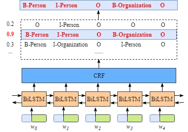
虽然不需要知道BiLSTM层的细节，但是为了更容易的理解CRF层，我们需要知道BiLSTM层输出的意义是什么。

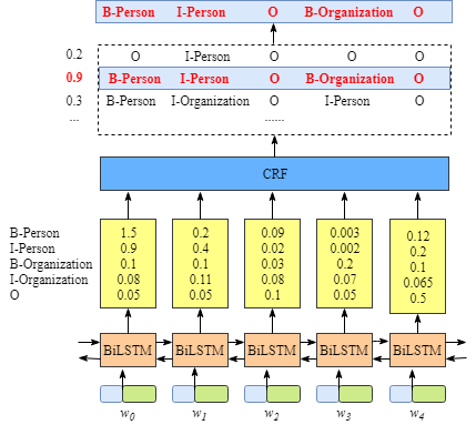
上图说明BiLSTM层的输出是每个标签的分数。例如，对于w0, BiLSTM节点的输出为1.5 (B-Person)、0.9 (I-Person)、0.1 (B-Organization)、0.08 (I-Organization)和0.05 (O)，这些分数将作为CRF层的输入。
然后，将BiLSTM层预测的所有分数输入CRF层。在CRF层中，选择预测得分最高的标签序列作为最佳答案。

为什么需要添加CRF层？

你可能已经发现，即使没有CRF层，也就是说，我们可以训练一个BiLSTM命名实体识别模型，如下图所示。

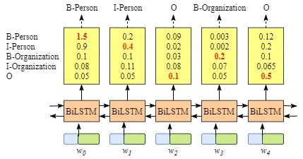
因为每个单词的BiLSTM的输出是标签分数。我们可以选择每个单词得分最高的标签。例如，对于w0，“B-Person”得分最高(1.5)，因此我们可以选择“B-Person”作为其最佳预测标签。同样，我们可以为w1选择“I-Person”，为w2选择“O”，为w3选择“B-Organization”，为w4选择“O”。
虽然在这个例子中我们可以得到正确的句子x的标签，但是并不总是这样。再试一下下面图片中的例子。

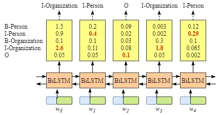
显然，这次的输出是无效的，“I-Organization I-Person”和“B-Organization I-Person”。

CRF层可以向最终的预测标签添加一些约束，以确保它们是有效的。这些约束可以由CRF层在训练过程中从训练数据集自动学习。
约束条件可以是：

• 句子中第一个单词的标签应该以“B-”或“O”开头，而不是“I-”
• “B-label1 I-label2 I-label3 I-…”，在这个模式中，label1、label2、label3…应该是相同的命名实体标签。例如，“B-Person I-Person”是有效的，但是“B-Person I-Organization”是无效的。
• “O I-label”无效。一个命名实体的第一个标签应该以“B-”而不是“I-”开头，换句话说，有效的模式应该是“O B-label”
• …

有了这些有用的约束，无效预测标签序列的数量将显著减少。

CRF层

在这一节中，我将分析CRF损失函数，来解释CRF层如何或为什么能够从训练数据集中学习上述约束。
在CRF层的损失函数中，我们有两种类型的分数。这两个分数是CRF层的关键概念。

Emission score

第一个是emission分数。这些emission分数来自BiLSTM层。例如，如图2.1所示，标记为B-Person的w0的分数为1.5。

为了方便起见，我们将给每个标签一个索引号，如下表所示。

我们用\(x_{iy_j}\)来表示emission分数。\(i\)是word的索引，\(y_j\)是label的索引。如图2.1所示，\(x_{i=1,y_j=2} = x_{w_1,B-Organization} = 0.1\)，即 \(w_1\)作为B-Organization的得分为0.1。

Transition score

我们使用\(t_{y_iy_j}\)来表示transition分数。例如，\(t_{B-Person, I-Person} = 0.9\)表示标签的transition，\(B-Person \rightarrow I-Person\)得分为0.9。因此，我们有一个transition得分矩阵，它存储了所有标签之间的所有得分。
为了使transition评分矩阵更健壮，我们将添加另外两个标签，START和END。START是指一个句子的开头，而不是第一个单词。END表示句子的结尾。
下面是一个transition得分矩阵的例子，包括额外添加的START和END标签。

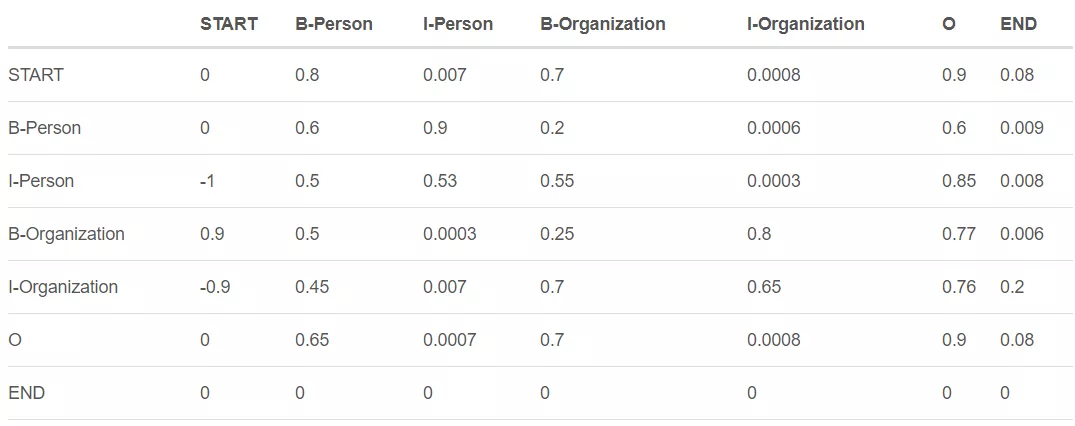
如上表所示，我们可以发现transition矩阵已经学习了一些有用的约束。

• 句子中第一个单词的标签应该以“B-”或“O”开头，而不是“I-”开头(从“START”到“I- person或I- organization”的transition分数非常低)
• “B-label1 I-label2 I-label3 I-…”，在这个模式中，label1、label2、label3…应该是相同的命名实体标签。例如，“B-Person I-Person”是有效的，但是“B-Person I-Organization”是无效的。(例如，从“B--- Organization”到“I-Person”的分数只有0.0003，比其他分数低很多)
• “O I-label”无效。一个被命名实体的第一个标签应该以“B-”而不是“I-”开头，换句话说，有效的模式应该是“O B-label”(同样，的分数非常小)
• …

你可能想问一个关于矩阵的问题。在哪里或如何得到transition矩阵？
实际上，该矩阵是BiLSTM-CRF模型的一个参数。在训练模型之前，可以随机初始化矩阵中的所有transition分数。所有的随机分数将在你的训练过程中自动更新。换句话说，CRF层可以自己学习这些约束。我们不需要手动构建矩阵。随着训练迭代次数的增加，分数会逐渐趋于合理。

CRF损失函数

CRF损失函数由真实路径得分和所有可能路径的总得分组成。在所有可能的路径中，真实路径的得分应该是最高的。
例如，如果我们的数据集中有如下表所示的这些标签：

我们还是有一个5个单词的句子。可能的路径是：

• 1. START B-Person B-Person B-Person B-Person B-Person END
• 2. START B-Person I-Person B-Person B-Person B-Person END
• …
• 10) START B-Person I-Person O B-Organization O END
• …
• N) O O O O O O O

假设每条可能的路径都有一个分数\(P_{i}\)，并且总共有\(N\)条可能的路径，所有路径的总分数是\(P_{total} = P_1 + P_2 + … + P_N = e^{S_1} + e^{S_2} + … + e^{S_N}\)。(在第2.4节中，我们将解释如何计算\(S_i\)，你也可以把它当作这条路径的分数。)
如果我们说第10条路径是真正的路径，换句话说，第10条路径是我们的训练数据集提供的黄金标准标签。在所有可能的路径中，得分\(P_{10}\)应该是百分比最大的。
在训练过程中，我们的BiLSTM-CRF模型的参数值将会一次又一次的更新，以保持增加真实路径的分数百分比。

\(Loss Function = \frac{P_{RealPath}}{P_1 + P_2 + … + P_N}\)

现在的问题是：

• 1)如何定义一个路径的分数？
• 2)如何计算所有可能路径的总分？
• 3)当我们计算总分时，我们需要列出所有可能的路径吗？(这个问题的答案是否定的.)

在下面的小节中，我们将看到如何解决这些问题。

实际路径得分

显然，在所有可能的路径中，一定有一条是真实路径。上节例子中句子的实际路径是“START B-Person I-Person O B-Organization O END”。其他的是不正确的，如“START B-Person B-Organization O I-Person I-Person B-Person”。\(e^{S_i}\)是第i条路径的得分。
在训练过程中，CRF损失函数只需要两个分数：真实路径的分数和所有可能路径的总分数。所有可能路径的分数中，真实路径分数所占的比例会逐渐增加。
计算实际路径分数\(e^{S_i}\)非常简单。这里我们主要关注的是\({S_i}\)的计算。
选取真实路径，“START B-Person I-Person O B-Organization O END”，我们以前用过，例如：

• 我们有一个5个单词的句子，w1,w2,w3,w4, w4,w5

• 我们增加了两个额外的单词来表示一个句子的开始和结束，w0,w6

• \({S_i}\)由两部分组成：\(S_i = EmissionScore + TransitionScore\)

Emission得分：
\(EmissionScore=x_{0,START}+x_{1,B-Person}+x_{2,I-Person}+x_{3,O}+x_{4,B-Organization}+x_{5,O}+x_{6,END}\)

• \(x_{index,label}\)是第index个单词被label标记的分数

• 这些得分$x_{1,B-Person} $ $ x_{2,I-Person} $ $ x_{3,O} $ $ x_{4,Organization} $ $ x_{5,O}$来自之前的BiLSTM输出。

• 对于\(x_{0,START}\)和\(x_{6,END}\)，我们可以把它们设为0。

Transition得分：

• \(t_{label1 \rightarrow label2}\)是从\(label1\)到\(label2\)的transition分数
• 这些分数来自CRF层。换句话说，这些transition分数实际上是CRF层的参数。

综上所述，现在我们可以计算出\(S_i\)以及路径得分\(e^{S_i}\)。

所有可能的路径的总得分

衡量总分最简单的方法是：列举所有可能的路径并将它们的分数相加。是的，你可以用这种方法计算总分。然而，这是非常低效的。训练的时间将是难以忍受的。下面我们将会通过一个toy例子，如何逐步计算一个句子的所有可能的路径的总分。下面我们开始在探索吧。

步骤1: 回想一下CRF损失函数
之前，我们将CRF损失函数定义为：

\(Loss Function = \frac{P_{RealPath}}{P_1 + P_2 + … + P_N}\)

现在我们把loss函数改变为对数loss函数：

\(LogLossFunction = \log \frac{P_{RealPath}}{P_1 + P_2 + … + P_N}\)

当我们训练一个模型时，通常我们的目标是最小化我们的损失函数，因此我们加上一个负号：

\(Log Loss Function = - \log \frac{P_{RealPath}}{P_1 + P_2 + … + P_N}\)

\(= - \log \frac{e^{S_{RealPath}}}{e^{S_1} + e^{S_2} + … + e^{S_N}}\)

\(= - (\log(e^{S_{RealPath}}) - \log(e^{S_1} + e^{S_2} + … + e^{S_N}))\)

\(= - (S_{RealPath} - \log(e^{S_1} + e^{S_2} + … + e^{S_N}))\)

\(= - ( \sum_{i=1}^{N} x_{iy_i} + \sum_{i=1}^{N-1} t_{y_iy_{i+1}} - \log(e^{S_1} + e^{S_2} + … + e^{S_N}))\)

在上一节中，我们已经知道如何计算实际路径得分，现在我们需要找到一个有效的解决方案来计算\(\log(e^{S_1} + e^{S_2} + … + e^{S_N})\)

步骤2: 回忆一下Emission和Transition得分
为了简化，我们假设我们从这个toy句子中训练我们的模型，它的长度只有3：
\(\mathbf{x} = [w_0, w_1, w_2]\)
此外，在我们的数据集中，我们有两个标签：
\(LabelSet = \{l_1,l_2\}\)
我们还有Bi-LSTM层输出的Emission分数：

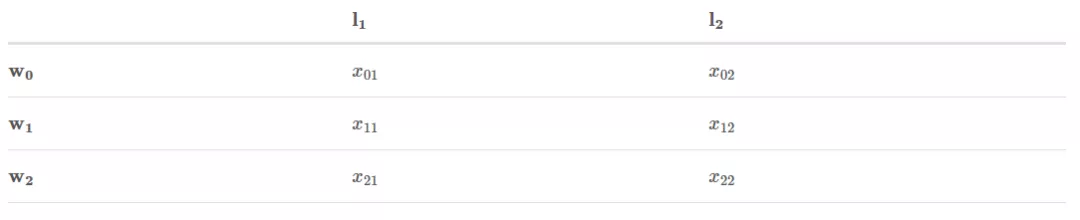
\(x_{ij}\)表示\(w_i\)被标记为\(l_j\)的得分。
此外，还有来自CRF层的Transition分数：

\(t_{ij}\)是从标签i到标签j的transition得分。

步骤3: 开始战斗（准备好纸笔）:
Remeber: Our goal is: \(log(e^{S1}+e^{S2}+…+e^{SN})\)

---

这个过程就是分数的累加。其思想与动态规划相似。简而言之，计算w0的所有可能路径的总分。然后，我们用总分来计算w0→w1。最后，我们使用最新的总分来计算w0→w1→w2。我们需要的是最后的总分。 在接下来的步骤中，你将看到两个变量：obs和previous。previous存储前面步骤的最终结果。obs表示当前单词的信息。

• previous：是一个向量，维数为标签tag的个数，每一维存储的是上一个位置所有的以某个tag为结尾的路径总分数的log之后的值
• obs：是一个向量，维数为标签tag的个数，每一维存储的是当前位置所对应的为某个tag的emission score。

---

w0:

\(obs = [x_{01}, x_{02}]\)
\(previous = None\)

如果我们的句子只有一个单词\(w_0\)，我们就没有前面步骤的结果，因此\(previous\)是\(None\)。另外，我们只能观察到第一个词\(obs = [x_{01}, x_{02}]\)。\(x_{01}\)和\(x_{02}\)是上述的Emission分数。
你可能会想，\(w_0\)的所有可能路径的总分是多少？答案很简单：

\(TotalScore(w_0)=\log (e^{x_{01}} + e^{x_{02}})\)

---

w0 \(\rightarrow\) w1:

\(obs = [x_{11}, x_{12}]\)
\(previous = [x_{01}, x_{02}]\)

1)把previous展开成：

\(previous =\left( \begin{matrix} x_{01}&x_{01}\\x_{02}&x_{02} \end{matrix} \right)\)

2)把obs展开成：
\(obs =\left( \begin{matrix} x_{11}&x_{12}\\ x_{11}&x_{12} \end{matrix} \right)\)

你可能想知道，为什么我们需要把previous和obs扩展成矩阵。因为矩阵可以提高计算的效率。在下面的过程中，你将很快看到这一点。
3)对 previous, obs以及transition得分求和：
\(scores =\left( \begin{matrix} x_{01}&x_{01}\\x_{02}&x_{02} \end{matrix} \right) + \left( \begin{matrix} x_{11}&x_{12}\\x_{11}&x_{12} \end{matrix} \right) + \left( \begin{matrix} t_{11}&t_{12}\\t_{21}&t_{22} \end{matrix} \right)\)

然后：
\(scores =\left( \begin{matrix} x_{01}+x_{11}+t_{11}&x_{01}+x_{12}+t_{12}\\ x_{02}+x_{11}+t_{21}&x_{02}+x_{12}+t_{22} \end{matrix} \right)\)

为下一个迭代修改previous的值：
\(previous=[\log (e^{x_{01}+x_{11}+t_{11}} + e^{x_{02}+x_{11}+t_{21}}), \log (e^{x_{01}+x_{12}+t_{12}} + e^{x_{02}+x_{12}+t_{22}})]\)

实际上，第二次迭代已经完成。如果有人想知道如何计算所有可能路径的总分(\(label_1\) \(\rightarrow\) \(label_1\), \(label_1\) \(\rightarrow\) \(label_2\), \(label_2\) \(\rightarrow\) \(label_1\), \(label_2\) \(\rightarrow\) \(label_2\))，从\(w_0\)到\(w_1\)，可以做如下计算。

我们使用新的previous中的元素：

\(TotalScore(w_0 \rightarrow w_1)\)
\( =\log (e^{previous[0]} + e^{previous[1]})\)
\( =\log (e^{\log(e^{x_{01}+x_{11}+t_{11}} + e^{x_{02}+x_{11}+t_{21}})}+e^{\log(e^{x_{01}+x_{12}+t_{12}} + e^{x_{02}+x_{12}+t_{22}})})\)
\( =\log(e^{x_{01}+x_{11}+t_{11}}+e^{x_{02}+x_{11}+t_{21}}+e^{x_{01}+x_{12}+t_{12}}+e^{x_{02}+x_{12}+t_{22}})\)

你发现了吗？这正是我们的目标：\(\log(e^{S_1} + e^{S_2} + … + e^{S_N})\)
在这个等式中，我们可以看到：

• \(S_1 = x_{01}+x_{11}+t_{11}\) (\(label_1\) → \(label_1\))
• \(S_2 = x_{02}+x_{11}+t_{21}\) (\(label_2\) → \(label_1\))
• \(S_3 = x_{01}+x_{12}+t_{12}\) (\(label_1\) → \(label_2\))
• \(S_4 = x_{02}+x_{12}+t_{22}\) (\(label_2\) → \(label_2\))

---

w0 → w1 → w2:

如果你读到这里了，你已经快要读完了，实际上，在这个迭代里，我们做的事情是和上个迭代一样的。
\(obs = [x_{21}, x_{22}]\)
\(previous=[\log (e^{x_{01}+x_{11}+t_{11}} + e^{x_{02}+x_{11}+t_{21}}), \log (e^{x_{01}+x_{12}+t_{12}} + e^{x_{02}+x_{12}+t_{22}})]\)

1)把previous扩展成：
\(previous =\left( \begin{matrix} \log (e^{x_{01}+x_{11}+t_{11}} + e^{x_{02}+x_{11}+t_{21}})&\log (e^{x_{01}+x_{11}+t_{11}} + e^{x_{02}+x_{11}+t_{21}})\\ \log (e^{x_{01}+x_{12}+t_{12}} + e^{x_{02}+x_{12}+t_{22}})&\log (e^{x_{01}+x_{12}+t_{12}} + e^{x_{02}+x_{12}+t_{22}}) \end{matrix} \right)\)

2)把obs扩展成：
\(obs =\left( \begin{matrix} x_{21}&x_{22}\\ x_{21}&x_{22} \end{matrix} \right)\)

3)把previous, obs和transition分数加起来:
\(scores = \left( \begin{matrix} \log (e^{x_{01}+x_{11}+t_{11}} + e^{x_{02}+x_{11}+t_{21}})&\log (e^{x_{01}+x_{11}+t_{11}} + e^{x_{02}+x_{11}+t_{21}})\\ \log (e^{x_{01}+x_{12}+t_{12}} + e^{x_{02}+x_{12}+t_{22}})&\log (e^{x_{01}+x_{12}+t_{12}} + e^{x_{02}+x_{12}+t_{22}}) \end{matrix} \right) + \left( \begin{matrix} x_{21}&x_{22}\\ x_{21}&x_{22} \end{matrix} \right) + \left( \begin{matrix} t_{11}&t_{12}\\ t_{21}&t_{22} \end{matrix} \right)\)

然后：
\(scores = \left( \begin{matrix} \log (e^{x_{01}+x_{11}+t_{11}} + e^{x_{02}+x_{11}+t_{21}}) + x_{21} + t_{11} &\log (e^{x_{01}+x_{11}+t_{11}} + e^{x_{02}+x_{11}+t_{21}}) + x_{22} + t_{12}\\ \log (e^{x_{01}+x_{12}+t_{12}} + e^{x_{02}+x_{12}+t_{22}}) + x_{21} + t_{21} &\log (e^{x_{01}+x_{12}+t_{12}} + e^{x_{02}+x_{12}+t_{22}}) + x_{22} + t_{22} \end{matrix} \right)\)

为下一轮迭代改变previous的值：
\(previous=[\) \(\log( e^{\log (e^{x_{01}+x_{11}+t_{11}} + e^{x_{02}+x_{11}+t_{21}}) + x_{21} + t_{11}} + e^{\log (e^{x_{01}+x_{12}+t_{12}} + e^{x_{02}+x_{12}+t_{22}}) + x_{21} + t_{21}} )\),\(\log( e^{\log (e^{x_{01}+x_{11}+t_{11}} + e^{x_{02}+x_{11}+t_{21}}) + x_{22} + t_{12}} + e^{\log (e^{x_{01}+x_{12}+t_{12}} + e^{x_{02}+x_{12}+t_{22}}) + x_{22} + t_{22}})\)]

\(=[\log((e^{x_{01}+x_{11}+t_{11}} + e^{x_{02}+x_{11}+t_{21}})e^{x_{21} + t_{11}}+(e^{x_{01}+x_{12}+t_{12}} + e^{x_{02}+x_{12}+t_{22}})e^{x_{21} + t_{21}}),\log((e^{x_{01}+x_{11}+t_{11}} + e^{x_{02}+x_{11}+t_{21}})e^{x_{22} + t_{12}}+(e^{x_{01}+x_{12}+t_{12}} + e^{x_{02}+x_{12}+t_{22}})e^{x_{22} + t_{22}})]\)

就像上一个迭代描述的一样，我们使用新的previous中的元素来计算总分数：
\(TotalScore(w_0 \rightarrow w_1 \rightarrow w_2)\)
\(=\log (e^{previous[0]} + e^{previous[1]})\)
\(=\log (e^{\log((e^{x_{01}+x_{11}+t_{11}} + e^{x_{02}+x_{11}+t_{21}})e^{x_{21} + t_{11}}+(e^{x_{01}+x_{12}+t_{12}} + e^{x_{02}+x_{12}+t_{22}})e^{x_{21} + t_{21}})}+e^{\log((e^{x_{01}+x_{11}+t_{11}} + e^{x_{02}+x_{11}+t_{21}})e^{x_{22} + t_{12}}+(e^{x_{01}+x_{12}+t_{12}} + e^{x_{02}+x_{12}+t_{22}})e^{x_{22} + t_{22}})})\)
\(=\log (e^{x_{01}+x_{11}+t_{11}+x_{21}+t_{11}}+e^{x_{02}+x_{11}+t_{21}+x_{21}+t_{11}}+e^{x_{01}+x_{12}+t_{12}+x_{21}+t_{21}}+e^{x_{02}+x_{12}+t_{22}+x_{21}+t_{21}}+e^{x_{01}+x_{11}+t_{11}+x_{22}+t_{12}}+e^{x_{02}+x_{11}+t_{21}+x_{22}+t_{12}}+e^{x_{01}+x_{12}+t_{12}+x_{22}+t_{22}}+e^{x_{02}+x_{12}+t_{22}+x_{22}+t_{22}})\)

我们达到了目标，\(\log(e^{S_1} + e^{S_2} + … + e^{S_N})\).我们的toy句子有三个单词，label set有两个label，所以一共应该有8种可能的label path。

---

虽然这个过程相当复杂，但是实现这个算法要容易得多。使用计算机的优点之一是可以完成一些重复性的工作。

为新的句子推断标签(维特比解码)

在前面的章节中，我们学习了BiLSTM-CRF模型的结构和CRF损失函数的细节。你可以通过各种开源框架(Keras、TensorFlow、pytorch等)实现自己的BiLSTM-CRF模型。最重要的事情之一是模型的反向传播是在这些框架上自动计算的，因此你不需要自己实现反向传播来训练你的模型(即计算梯度和更新参数)。此外，一些框架已经实现了CRF层，因此将CRF层与你自己的模型结合起来非常容易，只需添加一行代码即可。

在本节中，我们将探索如何在模型准备好时在测试期间推断句子的标签。

步骤1：BiLSTM-CRF模型的Emission和transition得分
假设，我们有一个包含三个单词的句子：\(\mathbf{x} = [w_0, w_1, w_2]\)
此外，我们已经从BiLSTM模型得到了Emission分数，从下面的CRF层得到了transition分数：

	l1	l2
w0	x01	x02
w1	x11	x12
w2	x21	x22

\(x_{ij}\)表示\(w_i\)被标记为\(l_j\)的得分。

	l1	l2
l1	t11	t12
l2	t21	t22

\(t_{ij}\)是从标签i转换成标签j的得分。

步骤2：开始推断

---

如果你熟悉Viterbi算法，那么这一部分对你来说很容易。但如果你不熟悉，请不要担心。与前一节类似，我将逐步解释该算法(先进行一个从左到右的前向过程，再从右到左进行回溯)。我们将从句子的左到右进行推断算法，如下所示：

• w0
• w0 → w1
• w0 → w1 → w2

你会看到两个变量：obs和previous。previous存储前面步骤的最终结果。obs表示当前单词的信息。
\(\mathbf{alpha_0}\)是历史最好得分，\(\mathbf{alpha_1}\)是历史对应的索引。这两个变量的细节将在它们出现时进行解释(方便我们进行回溯)。

---

w0:

\(obs = [x_{01}, x_{02}]\)
\(previous = None\)

现在，我们观察第一个单词\(w_{0}\)，目前为止，\(w_{0}\)最好的标签是很明显的。
比如，如果\(obs = [x_{01}=0.2, x_{02}=0.8]\)，很显然，\(w_{0}\)的最佳的标签是\(l_2\)。
因为只有一个单词，而且没有标签直接的转换，transition的得分没有用到。

---

w0 → w1:
\(obs = [x_{11}, x_{12}]\)
\(previous = [x_{01}, x_{02}]\)

1)把previous扩展成：
\(previous = \left( \begin{matrix} previous[0]&previous[0]\\ previous[1]&previous[1] \end{matrix} \right)= \left( \begin{matrix} x_{01}&x_{01}\\ x_{02}&x_{02} \end{matrix} \right)\)

2)把obs扩展成：
\(obs = \left( \begin{matrix} obs[0]&obs[1]\\ obs[0]&obs[1] \end{matrix} \right)= \left( \begin{matrix} x_{11}&x_{12}\\ x_{11}&x_{12} \end{matrix} \right)\)

3)把previous, obs和transition 分数都加起来：
\(scores = \left( \begin{matrix} x_{01}&x_{01}\\ x_{02}&x_{02} \end{matrix} \right) + \left( \begin{matrix} x_{11}&x_{12}\\ x_{11}&x_{12} \end{matrix} \right) + \left( \begin{matrix} t_{11}&t_{12}\\ t_{21}&t_{22} \end{matrix} \right)\)

然后：
\(scores = \left( \begin{matrix} x_{01}+x_{11}+t_{11}&x_{01}+x_{12}+t_{12}\\ x_{02}+x_{11}+t_{21}&x_{02}+x_{12}+t_{22} \end{matrix} \right)\)

你可能好奇，当我们计算所有路径的总分时，与上一节没有什么不同。请耐心和细心，你很快就会看到区别。
为下一次迭代更改previous的值：

\(previous=[\max (scores[00], scores[10]),\max (scores[01],scores[11])]\)

比如，如果我们的得分是：
\(scores = \left( \begin{matrix} x_{01}+x_{11}+t_{11}&x_{01}+x_{12}+t_{12}\\ x_{02}+x_{11}+t_{21}&x_{02}+x_{12}+t_{22} \end{matrix} \right)\) \(= \left( \begin{matrix} 0.2&0.3\\ 0.5&0.4 \end{matrix} \right)\)

我们的下个迭代的previous是：
\(previous=[\max (scores[00], scores[10]),\max (scores[01],scores[11])] = [0.5, 0.4]\)

previous列表存储了当前单词的每个标签的最大得分。

[Example Start]

举个例子：
我们知道在我们的语料中，我们总共只有2个标签，\(label1(l_1)\)和\(label2(l_2)\)。这两个标签的索引分别是0和1(因为在程序中index从0开始而不是1)。
\(previous[0]\)是以第0个标签\(l_1\)为结尾的路径的最大得分，类似的previous[1]是以第1个标签\(l_2\)为结尾的路径的最大得分。在每个迭代中，变量previous存储了以每个标签为结尾的路径的最大得分。换句话说，在每个迭代中，我们只保留了每个标签的最佳路径的信息 \((previous=[max(scores[00],scores[10]),max(scores[01],scores[11])])\)
具有小得分的路径信息会被丢掉。

[Example End]

回到我们的主任务：
同时，我们还有两个变量用来存储历史信息（得分和索引），\(alpha_0\)和\(alpha_1\)。
在这个迭代中，我们把最佳得分放入\(alpha_0\)，为了方便，每个标签的最大得分会加上下划线。

\(scores = \left( \begin{matrix} x_{01}+x_{11}+t_{11}&x_{01}+x_{12}+t_{12}\\ \underline{x_{02}+x_{11}+t_{21}}&\underline{x_{02}+x_{12}+t_{22}} \end{matrix} \right)= \left( \begin{matrix} 0.2&0.3\\ \underline{0.5}&\underline{0.4} \end{matrix} \right)\)

\(alpha_0=[(scores[10],scores[11])]=[(0.5,0.4)]\)

另外，对应的列的索引(当前词前一个词的状态的index)存在\(alpha_1\)里。

\(alpha_1=[(ColumnIndex(scores[10]),ColumnIndex(scores[11]))]=[(1,1)]\)

说明一下，\(l_1\)的索引是0，\(l_2\)的索引是1，所以\((1,1)=(l_2,l_2)\)表示,对于当前的单词\(w_i\)和标签\(l^{(i)}\):
当路径是\(\underline{l^{(i-1)}=l_2}\) → \(\underline{l^{(i)}=l_1}\)的时候，我们可以得到最大的得分是0.5，当路径是\(\underline{l^{(i-1)}=l_2}\) → \(\underline{l^{(i)}=l_2}\)的时候，我们可以得到最大的得分是0.4。\(l^{(i-1)}\)是前一个单词\(w_{i-1}\)的标签。

---

w0 → w1 → w2:

\(obs = [x_{21}, x_{22}]\)
\(previous = [0.5, 0.4]\)

1)把previous扩展成：
\(previous = \left( \begin{matrix} previous[0]&previous[0]\\ previous[1]&previous[1] \end{matrix} \right)= \left( \begin{matrix} 0.5&0.5\\ 0.4&0.4 \end{matrix} \right) \)

2)把obs扩展成：
\(obs = \left( \begin{matrix} obs[0]&obs[1]\\ obs[0]&obs[1] \end{matrix} \right)= \left( \begin{matrix} x_{21}&x_{22}\\ x_{21}&x_{22} \end{matrix} \right)\)

3)把previous, obs和transition 分数都加起来：
\(scores = \left( \begin{matrix} 0.5&0.5\\ 0.4&0.4 \end{matrix} \right) + \left( \begin{matrix} x_{21}&x_{22}\\ x_{21}&x_{22} \end{matrix} \right) + \left( \begin{matrix} t_{11}&t_{12}\\ t_{21}&t_{22} \end{matrix} \right)\)

然后：
\(scores = \left( \begin{matrix} 0.5+x_{11}+t_{11}&0.5+x_{12}+t_{12}\\ 0.4+x_{11}+t_{21}&0.4+x_{12}+t_{22} \end{matrix} \right)\)

为下一次迭代改变previous的值：

\(previous=[\max (scores[00], scores[10]),\max (scores[01],scores[11])]\)

Let’s say,这次迭代我们得到的分数是：

\(scores = \left( \begin{matrix} 0.6&\underline{0.9}\\ \underline{0.8}&0.7 \end{matrix} \right)\)

我们得到最新的previous：
\(previous=[0.8,0.9]\)
实际上，previous[0]和previous[1]中最大的那个就是预测的最佳路径。
同时，每个标签的最大分数和对应的索引会添加到\(alpha_0\)上和\(alpha_1\)上。

\(alpha_0=[(0.5,0.4),\underline{(scores[10],scores[01])}]\)
\(=[(0.5,0.4),\underline{(0.8,0.9)}]\)
\(alpha_1=[(1,1),\underline{(1,0)}]\)

步骤3：找到具有最高得分的最佳路径
这是最后一步,在此步骤中，将使用\(alpha_0\)和\(alpha_1\)来查找得分最高的路径。我们将从最后一个到第一个地去检查这两个列表中的元素。

---

\(w_1\) → \(w_2\):
首先，检查\(alpha_0\)和\(alpha_1\)的最后一个元素：\((0.8,0.9)\)和\((1,0)\)。0.9表示当label为\(l_2\)时，我们可以得到最高的路径分数0.9。我们还知道\(l_2\)的索引是1，因此检查\((1,0)[1]=0\)的值。索引“0”表示前一个标签为 \(l_1\)(\(l_1\)的索引为0)，因此我们可以得到 \(w_1\) → \(w_2\)的最佳路径：是\(l_1\) → \(l_2\)。

\(w_0\) → \(w_1\):

然后，我们继续向回移动并从\(alpha_1\)中得到元素：\((1,1)\)。从上一段我们知道\(w_1\)的label是\(l_1\)(index是0)，因此我们可以检查\((1,1)[0]=1\)。因此，我们可以得到这部分(\(w_0\) → \(w_1\))的最佳路径: \(l_2\) → \(l_1\)。

最后，我们这个例子中的最佳路径是\(l_2\) → \(l_1\) → \(l_2\)。

pytorch实现

上面已经把BiLSTM+CRF讲的清清楚楚了，光看理论还不够，我们要深入代码实战环节。

我们首先导入相应的包和定义一些后面要用到的辅助函数，如下，

import torch
import torch.nn as nn
import torch.optim as optim

torch.manual_seed(1)

# some helper functions
def argmax(vec):
    # return the argmax as a python int
    # 第1维度上最大值的下标
    # input: tensor([[2,3,4]])
    # output: 2
    _, idx = torch.max(vec,1)
    return idx.item()

def prepare_sequence(seq,to_ix):
    # 文本序列转化为index的序列形式
    idxs = [to_ix[w] for w in seq]
    return torch.tensor(idxs, dtype=torch.long)

# 这个函数的作用等价于torch.log(torch.sum(torch.exp(vec)))
def log_sum_exp(vec):
    #compute log sum exp in a numerically stable way for the forward algorithm
    # input: tensor([[2,3,4]])
    # max_score_broadcast: tensor([[4,4,4]])
    max_score = vec[0, argmax(vec)]
    max_score_broadcast = max_score.view(1,-1).expand(1,vec.size()[1])
    return max_score+torch.log(torch.sum(torch.exp(vec-max_score_broadcast)))

这里定义的几个辅助函数都比较直观，唯独log_sum_exp可能会对大家造成一点困扰，但其实这是一种考虑数值稳定性的求解办法，具体大家参考这篇博文即可。

我们接着看模型的定义，

# create model
class BiLSTM_CRF(nn.Module):
    def __init__(self,vocab_size, tag2ix, embedding_dim, hidden_dim):
        super(BiLSTM_CRF,self).__init__()
        self.embedding_dim = embedding_dim
        self.hidden_dim = hidden_dim
        self.tag2ix = tag2ix
        self.tagset_size = len(tag2ix)
        # 这里的单词嵌入矩阵是真实的单词嵌入矩阵，不包含在句子开始和结尾添加的人为的开始单词、结束单词
        self.word_embeds = nn.Embedding(vocab_size, embedding_dim)
        # LSTM默认数据格式batch_first = false
        self.lstm = nn.LSTM(embedding_dim, hidden_dim//2, num_layers=1, bidirectional=True)

        # maps output of lstm to tog space
        # 也即每个单词产生的Emission(发射) Score分布包含产生"<s>"和"<e>"的概率
        self.hidden2tag = nn.Linear(hidden_dim, self.tagset_size)

        # matrix of transition parameters
        # entry i, j is the score of transitioning to i from j
        # 所以，transition矩阵的每一列的元素之和为1
        # tag间的转移矩阵，是CRF层的参数
        # 这个transition矩阵包括"<s>" tag,"<e>" tag
        self.transitions = nn.Parameter(torch.randn(self.tagset_size, self.tagset_size))

        # these two statements enforce the constraint that we never transfer to the start tag
        # and we never transfer from the stop tag
        self.transitions.data[tag2ix[START_TAG], :] = -10000
        self.transitions.data[:, tag2ix[END_TAG]] = -10000
        
        self.hidden = self.init_hidden()
    # 作为lstm刚开始输入时的初值(h_0,c_0)，为一个元组
    # 初值的维数为num_layers * num_directions, batch, hidden_size
    # 说明一批中训练计算时用的是一样的h_0,c_0，不同批次使用的是不同的h_0,c_0
    def init_hidden(self):
        return (torch.randn(2, 1,self.hidden_dim//2),
                torch.randn(2, 1,self.hidden_dim//2))
    
    # 求log(e^s1 + e^s2 + e^s3 + ... + e^sN)的值，应用动态归化算法
    def _forward_alg(self, feats):
        # Do the forward algorithm to compute the partition(分治) function
        init_alphas = torch.full((1,self.tagset_size), -10000.)# tensor([[-10000.,-10000.,-10000.,-10000.,-10000.]])
        # START_TAG has all of the score
        init_alphas[0][self.tag2ix[START_TAG]] = 0#tensor([[-10000.,-10000.,-10000.,0,-10000.]])
        # Wrap in a variable so that we will get automatic backprop
        forward_var = init_alphas
        # Iterate through the sentence
        for feat in feats:
            #feat指Bi-LSTM模型每一步的输出，大小为tagset_size
            alphas_t = []# The forward tensors at this timestep
            for next_tag in range(self.tagset_size):
                # broadcast the emission score: it is the same regardless of(不管) the previous tag
                emit_score = feat[next_tag].view(1,-1).expand(1,self.tagset_size)
                # the ith entry of trans_score is the score of transitioning to next_tag from i
                trans_score = self.transitions[next_tag].view(1,-1)
                # The ith entry of next_tag_var is the value for the
                # edge (i -> next_tag) before we do log-sum-exp
                next_tag_var = forward_var + trans_score + emit_score
                # The forward variable for this tag is log-sum-exp of all the
                # scores.
                alphas_t.append(log_sum_exp(next_tag_var).view(1))
            forward_var = torch.cat(alphas_t).view(1,-1)
        terminal_var = forward_var+self.transitions[self.tag2ix[END_TAG]]
        alpha = log_sum_exp(terminal_var)
        return alpha

    def _get_lstm_features(self,sentence):
        self.hidden = self.init_hidden()
        embeds = self.word_embeds(sentence).view(len(sentence),1,-1)
        lstm_out, self.hidden = self.lstm(embeds, self.hidden)
        lstm_out = lstm_out.view(len(sentence), self.hidden_dim)
        lstm_feats = self.hidden2tag(lstm_out)
        return lstm_feats

    def _score_sentence(self,feats,tags):
        # gives the score of a provides tag sequence
        # 求某一路径的值
        score = torch.zeros(1)
        tags = torch.cat([torch.tensor([self.tag2ix[START_TAG]], dtype=torch.long), tags])
        # feats中的i位置对应tags中的i+1位置
        # 这里的实现版本的emisson score为句子所有的真实单词位置的，不包含人为添加的START_TAG位置和END_TAG位置
        # 而transition score则包含START_TAG位置 -> 句子的第一个真实单词之间的转换分数
        # 和句子的最后一个真实单词 -> END_TAG位置之间的转换分数 
        for i , feat in enumerate(feats):
            score = score + self.transitions[tags[i + 1], tags[i]] + feat[tags[i + 1]]
        score = score + self.transitions[self.tag2ix[END_TAG], tags[-1]]
        return score

    def _viterbi_decode(self, feats):
        backpointers = []
        # Initialize the viterbi variables in log space
        init_vars = torch.full((1,self.tagset_size),-10000.)# tensor([[-10000.,-10000.,-10000.,-10000.,-10000.]])
        init_vars[0][self.tag2ix[START_TAG]] = 0#tensor([[-10000.,-10000.,-10000.,0,-10000.]])
        # forward_var at step i holds the viterbi variables for step i-1
        forward_var = init_vars
        for feat in feats:
            bptrs_t = [] # holds the back pointers for this step
            viterbivars_t = [] # holds the viterbi variables for this step

            for next_tag in range(self.tagset_size):
                # next_tag_var[i] holds the viterbi variable for tag i at the
                # previous step, plus the score of transitioning
                # from tag i to next_tag.
                # We don't include the emission scores here because the max
                # does not depend on them (we add them in below)
                next_tag_var = forward_var + self.transitions[next_tag]
                best_tag_id = argmax(next_tag_var)
                bptrs_t.append(best_tag_id)
                viterbivars_t.append(next_tag_var[0][best_tag_id].view(1))
            # Now add in the emission scores, and assign forward_var to the set
            # of viterbi variables we just computed
            forward_var = (torch.cat(viterbivars_t) + feat).view(1, -1)
            backpointers.append(bptrs_t)

        # Transition to STOP_TAG
        terminal_var = forward_var + self.transitions[self.tag2ix[END_TAG]]
        best_tag_id = argmax(terminal_var)
        path_score = terminal_var[0][best_tag_id]

        # Follow the back pointers to decode the best path.
        best_path = [best_tag_id]
        for bptrs_t in reversed(backpointers):
            best_tag_id = bptrs_t[best_tag_id]
            best_path.append(best_tag_id)
        # Pop off the start tag (we dont want to return that to the caller)
        start = best_path.pop()
        assert start == self.tag2ix[START_TAG]  # Sanity check
        best_path.reverse()
        return path_score, best_path
    # 注意，这里的实现为单个句子版本，不是批版本
    def neg_log_likelihood(self, sentence, tags):
        # 由lstm层计算得的每一时刻属于某一tag的值
        feats = self._get_lstm_features(sentence)
        # log(e^s1 + e^s2 + e^s3 + ... + e^sN)
        forward_score = self._forward_alg(feats)
        # 正确路径的值，s_realpath
        gold_score = self._score_sentence(feats, tags)
        # -(s_realpath - log(e^s1 + e^s2 + e^s3 + ... + e^sN)）
        return forward_score - gold_score

    def forward(self, sentence):  # dont confuse this with _forward_alg above.
        # Get the emission scores from the BiLSTM
        lstm_feats = self._get_lstm_features(sentence)

        # Find the best path, given the features.
        score, tag_seq = self._viterbi_decode(lstm_feats)
        return score, tag_seq

上面的注释应该说很详细了，只有CRF层是需要自己手写出来的。所以，大家重点关注一下_forward_alg这个函数，就是我们上面讲的求解\(\log(e^{S_1} + e^{S_2} + … + e^{S_N})\)的函数，关于这个函数的计算原理，上面已经通过例子展示过了，为了更清晰一点，这里把用动态规划时的递推公式原理写出来，以利于理解。
对于一个序列，假设它有N个解码路径，我们要求的是\(\log(e^{S_1} + e^{S_2} + … + e^{S_N})\)，直接求一个一个地算，太麻烦，复杂度很好，所以我们使用了动态规划的思想，逐个时间步的计算，在每个时间步t，我们维护一个长度为tag_size的向量\(cur^t\)(这里只是为了论述的方便，没用代码了的变量)，
\(cur^t[j] = logsumexp(S^t_1,S^t_2,S^t_3,...,S^t_{N_j})\)，其中\(S^t_1,S^t_2,S^t_3,...,S^t_{N_j}\)为从序列开始到此时间步t的所有路径中时间步t标签为j的路径的各自得分。则：


而我们最终要求的结果\(\log(e^{S_1} + e^{S_2} + … + e^{S_N})\)显然等于：
\(logsumexp(cur^{terminal})\)
terminal为最终时间步。

最后，我们再来看一下主函数，

if __name__ == "__main__":
    START_TAG = "<s>"
    END_TAG = "<e>"
    EMBEDDING_DIM = 5
    HIDDEN_DIM = 4

    # Make up some training data
    # 注意：这里的两个样本的长度不一样长
    training_data = [(
        "the wall street journal reported today that apple corporation made money".split(),
        "B I I I O O O B I O O".split()
    ), (
        "georgia tech is a university in georgia".split(),
        "B I O O O O B".split()
    )]
    # 构造单词->单词序号的映射字典(这个字典中不包括人为的句子开始单词："<START>"，以及人为的句子结束单词："<STOP>")
    word2ix = {}
    for sentence, tags in training_data:
        for word in sentence:
            if word not in word2ix:
                word2ix[word] = len(word2ix)

    tag2ix = {"B": 0, "I": 1, "O": 2, START_TAG: 3, END_TAG: 4}

    model = BiLSTM_CRF(len(word2ix), tag2ix, EMBEDDING_DIM, HIDDEN_DIM)
    optimizer = optim.SGD(model.parameters(), lr=0.01, weight_decay=1e-4)

    # Check predictions before training
    # 输出训练前的预测序列
    with torch.no_grad():
        precheck_sent = prepare_sequence(training_data[0][0], word2ix)
        precheck_tags = torch.tensor([tag2ix[t] for t in training_data[0][1]], dtype=torch.long)
        print(model(precheck_sent))

    # Make sure prepare_sequence from earlier in the LSTM section is loaded
    for epoch in range(300):  # again, normally you would NOT do 300 epochs, it is toy data
        for sentence, tags in training_data:
            # Step 1. Remember that Pytorch accumulates gradients.
            # We need to clear them out before each instance
            model.zero_grad()

            # Step 2. Get our inputs ready for the network, that is,
            # turn them into Tensors of word indices.
            # 注意：这里的model的输入sentence_in：句子的单词index序列没有经过额外的处理(人为地增加句子开始、结束单词)
            sentence_in = prepare_sequence(sentence, word2ix)
            # 训练时，句子的tags序列也没有经过额外的处理(人为地增加句子开始、结束tag)
            targets = torch.tensor([tag2ix[t] for t in tags], dtype=torch.long)

            # Step 3. Run our forward pass.
            loss = model.neg_log_likelihood(sentence_in, targets)

            # Step 4. Compute the loss, gradients, and update the parameters by
            # calling optimizer.step()
            loss.backward()
            optimizer.step()

    # Check predictions after training
    with torch.no_grad():
        precheck_sent = prepare_sequence(training_data[0][0], word2ix)
        print(model(precheck_sent))

    # 输出结果
    # (tensor(-9996.9365), [1, 2, 2, 2, 2, 2, 2, 2, 2, 2, 2])
    # (tensor(-9973.2725), [0, 1, 1, 1, 2, 2, 2, 0, 1, 2, 2])

参考

机器学习基础（11）条件随机场的理解及BI-LSTM+CRF实战
CRF Layer on the Top of BiLSTM