

(译)BERT Fine-Tuning Tutorial with PyTorch
本文原地址见这里,与本教程对应的 Colab Notebook的地址在这里,里面包含了完整的可运行的代码。
Introduction
History
2018 年是 NLP 突破的一年,迁移学习、特别是 Allen AI 的 ELMO,OpenAI 的 Open-GPT,以及 Google 的 BERT,这些模型让研究者们刷新了多项任务的基线(benchmark),并提供了容易被微调预训练模型(只需很少的数据量和计算量),使用它们,可产出当今最高水平的结果。但是,对于刚接触 NLP 甚至很多有经验的开发者来说,这些强大模型的理论和应用并不是那么容易理解。
What is BERT?
2018年底发布的BERT(Bidirectional Encoder Representations from Transformers)是我们在本教程中要用到的模型,目的是让读者更好地理解和指导读者在 NLP 中使用迁移学习模型。BERT是一种预训练语言表征的方法,NLP实践者可以免费下载并使用这些模型。你可以用这些模型从文本数据中提取高质量的语言特征,也可以用自己的数据对这些模型在特定的任务(分类、实体识别、问答问题等)上进行微调,以产生高质量的预测结果。本文将解释如何修改和微调 BERT,以创建一个强大的 NLP 模型。
Advantages of Fine-Tuning
在本教程中,我们将使用BERT来训练一个文本分类器。具体来说,我们将采取预训练的 BERT 模型,在末端添加一个未训练过的神经元层,然后训练新的模型来完成我们的分类任务。为什么要这样做,而不是训练一个特定的深度学习模型(CNN、BiLSTM等)?
- 更快速的开发
首先,预训练的 BERT 模型权重已经编码了很多关于我们语言的信息。因此,训练我们的微调模型所需的时间要少得多——就好像我们已经对网络的底层进行了广泛的训练,只需要将它们作为我们的分类任务的特征,并轻微地调整它们就好。事实上,作者建议在特定的 NLP 任务上对 BERT 进行微调时,只需要 2-4 个 epochs 的训练(相比之下,从头开始训练原始 BERT 或 LSTM 模型需要数百个 GPU 小时)。 - 更少的数据
此外,也许同样重要的是,预训练这种方法,允许我们在一个比从头开始建立的模型所需要的数据集小得多的数据集上进行微调。从零开始建立的 NLP 模型的一个主要缺点是,我们通常需要一个庞大的数据集来训练我们的网络,以达到合理的精度,这意味着我们必须投入大量的时间和精力在数据集的创建上。通过对 BERT 进行微调,我们现在可以在更少的数据集上训练一个模型,使其达到良好的性能。 - 更好的结果
最后,这种简单的微调程过程(通常在 BERT 的基础上增加一个全连接层,并训练几个 epochs)被证明可以在广泛的任务中以最小的调节代价来实现最先进的结果:分类、语言推理、语义相似度、问答问题等。与其实现定制的、有时还很难理解的网络结构来完成特定的任务,不如使用 BERT 进行简单的微调,也许是一个更好的(至少不会差)选择。
A Shift in NLP
这种向迁移学习的转变,与几年前计算机视觉领域发生的转变相似。为计算机视觉任务创建一个好的深度学习网络可能需要数百万个参数,并且训练成本非常高。研究人员发现,深度网络的特征表示可以分层进行学习(在最底层学习简单的特征,如物体边缘等,在更高的层逐渐增加复杂的特征)。与其每次从头开始训练一个新的网络,不如将训练好的网络的低层泛化图像特征复制并转移到另一个有不同任务的网络中使用。很快,下载一个预训练过的深度网络,然后为新任务快速地重新训练它,或者在上面添加额外的层,这已成为一种常见的做法——这比从头开始训练一个昂贵的网络要好得多。对许多人来说,2018年推出的深度预训练语言模型(ELMO、BERT、ULMFIT、Open-GPT等),预示着和计算机视觉一样,NLP 正在向迁移学习发生转变。
让我们开始吧!
1. Setup
1.1. Using Colab GPU for Training
Google Colab 提供免费的 GPU 和 TPU!由于我们将训练一个大型的神经网络,所以最好使用这些硬件加速(本文中,我们将使用一个 GPU),否则训练将需要很长时间。
你可以在目录中选择添加 GPU
Edit 🡒 Notebook Settings 🡒 Hardware accelerator 🡒 (GPU)
接着运行下面代码来确认 GPU 被检测到:
import torch

# If there's a GPU available...
if torch.cuda.is_available():

    # Tell PyTorch to use the GPU.
    device = torch.device("cuda")

    print('There are %d GPU(s) available.' % torch.cuda.device_count())

    print('We will use the GPU:', torch.cuda.get_device_name(0))

# If not...
else:
    print('No GPU available, using the CPU instead.')
    device = torch.device("cpu")
There are 1 GPU(s) available.
We will use the GPU: Tesla P100-PCIE-16GB
1.2. Installing the Hugging Face Library
下一步,我们来安装 Hugging Face 的 transformers 库,它将为我们提供一个 BERT 的 pytorch 接口(这个库包含其他预训练语言模型的接口,如 OpenAI 的 GPT 和 GPT-2)。我们选择了 pytorch 接口,因为它在高层次的API(很容易使用,但缺乏细节)和 tensorflow 代码(其中包含很多细节,这往往会让我们陷入关于 tensorflow 的学习中,而这里的目的是 BERT!)之间取得了很好的平衡。
目前来看,Hugging Face 似乎是被广泛接受的、最强大的 Bert 接口。除了支持各种不同的预训练模型外,该库还包含了适应于不同任务的模型的预构建。例如,在本教程中,我们将使用 BertForSequenceClassification 来做文本分类。
该库还为 token classification、question answering、next sentence prediction 等不同 NLP 任务提供特定的类库。使用这些预构建的类,可以简化定制 BERT 的过程。安装 transformer:
!pip install transformers
本教程中的代码实际上是 huggingface 样例代码 run_glue.py 的简化版本。run_glue.py 是一个有用的工具,它可以让你选择你想运行的 GLUE 任务,以及你想使用的预训练模型。它还支持使用 CPU、单个 GPU 或多个 GPU。如果你想进一步提高速度,它甚至支持使用 16 位精度。
遗憾的是,所有这些配置让代码的可读性变得很差,本教程会极大的简化这些代码,并增加大量的注释,让大家知其然,并知其所以然。
2. Loading CoLA Dataset
我们将使用 The Corpus of Linguistic Acceptability(CoLA)数据集进行单句分类。它是一组被标记为语法正确或错误的句子。它于2018年5月首次发布,是 "GLUE Benchmark" 中的数据集之一。
2.1. Download & Extract
我们使用 wget 来下载数据集,安装 wget:
!pip install wget
下载数据集:
import wget
import os

print('Downloading dataset...')

# The URL for the dataset zip file.
url = 'https://nyu-mll.github.io/CoLA/cola_public_1.1.zip'

# Download the file (if we haven't already)
if not os.path.exists('./cola_public_1.1.zip'):
    wget.download(url, './cola_public_1.1.zip')
解压之后,你就可以在 Colab 左侧的文件系统窗口看到这些文件:
# Unzip the dataset (if we haven't already)
if not os.path.exists('./cola_public/'):
    !unzip cola_public_1.1.zip
2.2. Parse
从解压后的文件名就可以看出哪些文件是分词后的,哪些是原始文件。
我们使用未分词版本的数据,因为要应用预训练 BERT,必须使用模型自带的分词器。这是因为: (1) 模型有一个固定的词汇表, (2) BERT 用一种特殊的方式来处理词汇外的单词(out-of-vocabulary)。
先使用 pandas 来解析 in_domain_train.tsv 文件,并预览这些数据:
import pandas as pd

# Load the dataset into a pandas dataframe.
df = pd.read_csv("./cola_public/raw/in_domain_train.tsv", delimiter='\t', header=None, names=['sentence_source', 'label', 'label_notes', 'sentence'])

# Report the number of sentences.
print('Number of training sentences: {:,}\n'.format(df.shape[0]))

# Display 10 random rows from the data.
df.sample(10)
Number of training sentences: 8,551
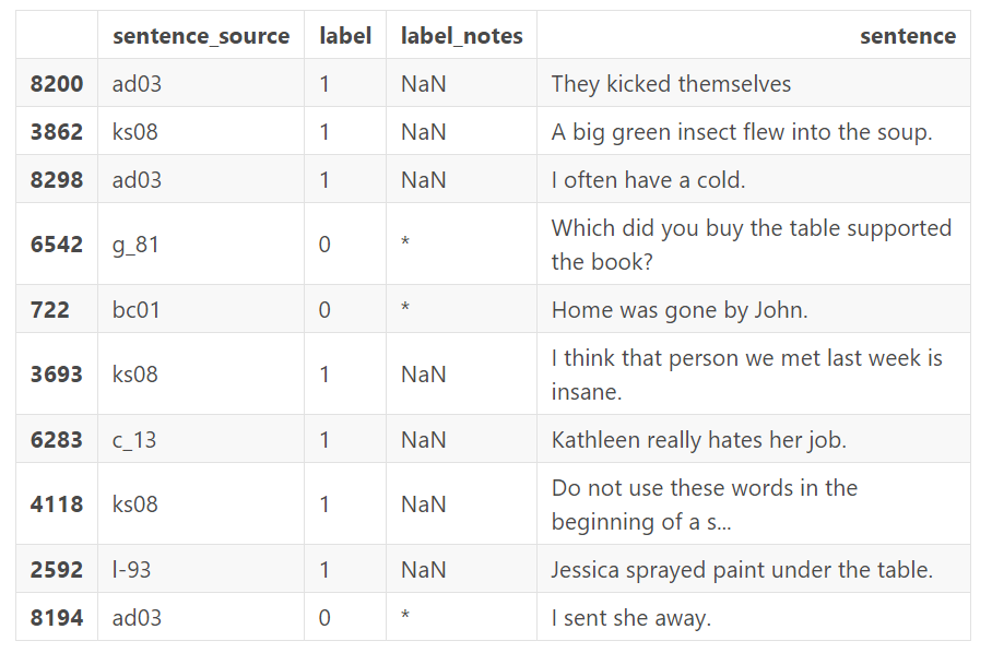
上表中我们主要关心 sentence 和 label 字段,label 中 0 表示“语法不可接受”,而 1 表示“语法可接受”。
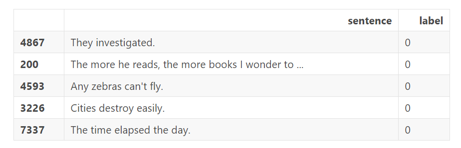
下面是 5 个语法上不可接受的例子,可以看到相对于情感分析来说,这个任务要困难很多:
df.loc[df.label == 0].sample(5)[['sentence', 'label']]
我们把 sentence 和 label 字段加载到 numpy 数组中
# Get the lists of sentences and their labels.
sentences = df.sentence.values
labels = df.label.values
3.Tokenization & Input Formatting
在本小节中,我们会将数据集转化为可以被BERT训练的格式。
3.1.BERT Tokenizer
要将文本输入到BERT中,必须先对它们分词,然后这些tokens一定要被映射到(mapped)分词器词汇表中的对应下标。这个分词操作,必须通过在我们下面将要下载的BERT里面包含的分词器下进行操作。这里我们使用"uncased" 版本的bert。(译者注:uncased版本是不能区分大小写,因为词汇表中只有小写,所以,在我们使用时需要指定do_lower_case=True参数。而cased版本能够区分大小写,不需要事先转化为小写。)
from transformers import BertTokenizer

# Load the BERT tokenizer.
print('Loading BERT tokenizer...')
tokenizer = BertTokenizer.from_pretrained('bert-base-uncased', do_lower_case=True)
让我们应用这个分词器在一个句子上,看一看输出。
# Print the original sentence.
print(' Original: ', sentences[0])

# Print the sentence split into tokens.
print('Tokenized: ', tokenizer.tokenize(sentences[0]))

# Print the sentence mapped to token ids.
print('Token IDs: ', tokenizer.convert_tokens_to_ids(tokenizer.tokenize(sentences[0])))
Original:  Our friends won't buy this analysis, let alone the next one we propose.
Tokenized:  ['our', 'friends', 'won', "'", 't', 'buy', 'this', 'analysis', ',', 'let', 'alone', 'the', 'next', 'one', 'we', 'propose', '.']
Token IDs:  [2256, 2814, 2180, 1005, 1056, 4965, 2023, 4106, 1010, 2292, 2894, 1996, 2279, 2028, 2057, 16599, 1012]
当我们实际转换所有的句子的时候,我们将使用tokenize.encode函数去处理这两步,而不是单独的去各自调用tokenize 和convert_tokens_to_ids 。在此之前,我们需要先谈论一下关于BERT的输入格式要求。
3.2.Required Formatting
我们被要求:
- 在句子的句首和句尾添加特殊的符号
- 给句子填充 or 截断,使每个句子保持固定的长度
- 用 “attention mask” 来显示的区分填充的 tokens 和非填充的 tokens。
Special Tokens
[SEP]
在每个句子的结尾,需要添加特殊的 [SEP] 符号。在以输入为两个句子的任务中(例如:句子 A 中的问题的答案是否可以在句子 B 中找到),该符号为这两个句子的分隔符。目前为止我还不清楚为什么我们仅有一个句子输入的情况下,仍然被要求加入该符号,但既然这样要求我们就这么做吧。
[CLS]
在分类任务中,我们需要将 [CLS] 符号插入到每个句子的开头。这个符号有特殊的意义,BERT 包含 12 个 Transformer 层,每层接受一组 token 的 embeddings 列表作为输入,并产生相同数目的 embeddings 作为输出(当然,它们的值是不同的)。
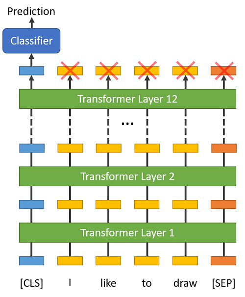
最后一层 transformer 的输出,只有第 1 个 embedding(对应到 [CLS] 符号)会输入到分类器中。
“The first token of every sequence is always a special classification token ([CLS]). The final hidden state corresponding to this token is used as the aggregate sequence representation for classification tasks.” (from the BERT paper)
Sentence Length & Attention Mask
我们数据集中的句子有各自不同的长度,那么BERT是怎么处理的呢?
- 所有句子必须被填充或截断到一个单独的、固定的长度,
- 句子最大的长度为 512 个 tokens。
填充句子要使用 [PAD] token,它在 BERT词汇表中的下标为 0,下图是最大长度为 8 个 tokens 的填充说明。
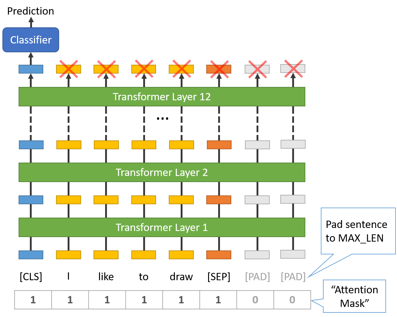
“Attention Mask” 是一个只有 0 和 1 组成的数组,标记哪些 tokens 是填充的,哪些不是的。这个掩码会告诉 BERT 中的 “Self-Attention” 机制,不要将这些PAD tokens纳入对句子的解释之中。
句子的最大长度配置会影响训练和评估速度,例如,在 Tesla K80 上有以下测试:
AX_LEN = 128 --> Training epochs take ~5:28 each

MAX_LEN = 64 --> Training epochs take ~2:57 each
3.3.Tokenize Dataset
transformers 库提供的 encode 函数会帮助我们处理大多数解析和数据预准备的工作。在encode文本之前,我们需要确定 MAX_LEN 这个参数,下面的代码可以计算数据集中句子的最大长度:
max_len = 0

# For every sentence...
for sent in sentences:

    # Tokenize the text and add `[CLS]` and `[SEP]` tokens.
    input_ids = tokenizer.encode(sent, add_special_tokens=True)

    # Update the maximum sentence length.
    max_len = max(max_len, len(input_ids))

print('Max sentence length: ', max_len)
Max sentence length:  47
为了避免不会出现更长的测试句子,这里我们将 MAX_LEN 设为 64。下面我们正式开始分词。
函数 tokenizer.encode_plus 为我们组合了多个步骤:
- 将句子分词为 tokens。
- 在两端添加特殊符号 [CLS] 和[SEP]。
- 将 tokens 映射为下标 IDs。
- 将列表填充或截断为固定的长度。
- 创建 attention masks,将填充的和非填充 tokens 区分开来。
前4个特征包含在tokenizer.encode函数中,但是这里我将使用tokenizer.encode_plus去得到第5个输出结果(attention masks).具体可以看出这里
# Tokenize all of the sentences and map the tokens to thier word IDs.
input_ids = []
attention_masks = []

# For every sentence...
for sent in sentences:
    # `encode_plus` will:
    #   (1) Tokenize the sentence.
    #   (2) Prepend the `[CLS]` token to the start.
    #   (3) Append the `[SEP]` token to the end.
    #   (4) Map tokens to their IDs.
    #   (5) Pad or truncate the sentence to `max_length`
    #   (6) Create attention masks for [PAD] tokens.
    encoded_dict = tokenizer.encode_plus(
                        sent,                      # Sentence to encode.
                        add_special_tokens = True, # Add '[CLS]' and '[SEP]'
                        max_length = 64,           # Pad & truncate all sentences.
                        pad_to_max_length = True,
                        return_attention_mask = True,   # Construct attn. masks.
                        return_tensors = 'pt',     # Return pytorch tensors.
                   )

    # Add the encoded sentence to the list.
    input_ids.append(encoded_dict['input_ids'])

    # And its attention mask (simply differentiates padding from non-padding).
    attention_masks.append(encoded_dict['attention_mask'])

# Convert the lists into tensors.
input_ids = torch.cat(input_ids, dim=0)
attention_masks = torch.cat(attention_masks, dim=0)
labels = torch.tensor(labels)

# Print sentence 0, now as a list of IDs.
print('Original: ', sentences[0])
print('Token IDs:', input_ids[0])
Original:  Our friends won't buy this analysis, let alone the next one we propose.
Token IDs: tensor([  101,  2256,  2814,  2180,  1005,  1056,  4965,  2023,  4106,  1010,
         2292,  2894,  1996,  2279,  2028,  2057, 16599,  1012,   102,     0,
            0,     0,     0,     0,     0,     0,     0,     0,     0,     0,
            0,     0,     0,     0,     0,     0,     0,     0,     0,     0,
            0,     0,     0,     0,     0,     0,     0,     0,     0,     0,
            0,     0,     0,     0,     0,     0,     0,     0,     0,     0,
            0,     0,     0,     0])
3.4.Training & Validation Split
将 90% 的数据集作为训练集,剩下的 10% 作为验证集:
from torch.utils.data import TensorDataset, random_split

# Combine the training inputs into a TensorDataset.
dataset = TensorDataset(input_ids, attention_masks, labels)

# Create a 90-10 train-validation split.

# Calculate the number of samples to include in each set.
train_size = int(0.9 * len(dataset))
val_size = len(dataset) - train_size

# Divide the dataset by randomly selecting samples.
train_dataset, val_dataset = random_split(dataset, [train_size, val_size])

print('{:>5,} training samples'.format(train_size))
print('{:>5,} validation samples'.format(val_size))
7,695 training samples
856 validation samples
我们也将使用torch中的DataLoader类,为我们的数据集创造一个迭代器,这会在我们训练的过程中,有助于节省内存。因为不像一个for循环,通过一个迭代器,整个数据集不需要被加载进内存。
from torch.utils.data import DataLoader, RandomSampler, SequentialSampler

# The DataLoader needs to know our batch size for training, so we specify it
# here. For fine-tuning BERT on a specific task, the authors recommend a batch
# size of 16 or 32.
batch_size = 32

# Create the DataLoaders for our training and validation sets.
# We'll take training samples in random order.
train_dataloader = DataLoader(
            train_dataset,  # The training samples.
            sampler = RandomSampler(train_dataset), # Select batches randomly
            batch_size = batch_size # Trains with this batch size.
        )

# For validation the order doesn't matter, so we'll just read them sequentially.
validation_dataloader = DataLoader(
            val_dataset, # The validation samples.
            sampler = SequentialSampler(val_dataset), # Pull out batches sequentially.
            batch_size = batch_size # Evaluate with this batch size.
        )
4. Train Our Classification Model
现在模型的输入数据已经被转换成了合适的输入格式,是时候开始微调BERT模型了。
4.1. BertForSequenceClassification
对于这个任务,我们首先要修改这个BERT预训练模型,让它的输出去分类,然后,我们在我们的数据集上继续训练这个模型,直到整个模型,端到端的,能很好的适用于我们的任务。
幸运的是,huggingface 的 pytorch 实现包含一系列接口,就是为不同的 NLP 任务设计的。这些接口无一例外的构建于 BERT 模型之上,对于不同的 NLP 任务,它们有不同的结构和不同的输出类型。
以下是当前提供给微调的类列表:
- BertModel
- BertForPreTraining
- BertForMaskedLM
- BertForNextSentencePrediction
- BertForSequenceClassification - The one we’ll use.
- BertForTokenClassification
- BertForQuestionAnswering
这些类的参考文档在这里。
我们将使用 BertForSequenceClassification,它由一个普通的 BERT 模型和一个额外的单线性层组成,而后者主要负责文本分类。当我们向模型输入数据时,整个预训练 BERT 模型和额外的未训练的分类层将在我们特定的任务上被训练。
好了, 我们现在加载 BERT!有几种不同的预训练模型可供选择,"bert-base-uncased" 是只有小写字母的版本,且它是 "base" 和 "large" 中的较小版。
from_pretrained 的参考文档在这里,额外的参数说明在这里。
from transformers import BertForSequenceClassification, AdamW, BertConfig

# Load BertForSequenceClassification, the pretrained BERT model with a single
# linear classification layer on top.
model = BertForSequenceClassification.from_pretrained(
    "bert-base-uncased", # Use the 12-layer BERT model, with an uncased vocab.
    num_labels = 2, # The number of output labels--2 for binary classification.
                    # You can increase this for multi-class tasks.
    output_attentions = False, # Whether the model returns attentions weights.
    output_hidden_states = False, # Whether the model returns all hidden-states.
)

# Tell pytorch to run this model on the GPU.
model.cuda()
好奇心使然,我们可以根据参数名来查看所有的模型参数。
下面会打印参数名和参数的维度:
- embedding 层
- 12 层 transformers 的第 1 层
- 输出层
# Get all of the model's parameters as a list of tuples.
params = list(model.named_parameters())

print('The BERT model has {:} different named parameters.\n'.format(len(params)))

print('==== Embedding Layer ====\n')

for p in params[0:5]:
    print("{:<55} {:>12}".format(p[0], str(tuple(p[1].size()))))

print('\n==== First Transformer ====\n')

for p in params[5:21]:
    print("{:<55} {:>12}".format(p[0], str(tuple(p[1].size()))))

print('\n==== Output Layer ====\n')

for p in params[-4:]:
    print("{:<55} {:>12}".format(p[0], str(tuple(p[1].size()))))
The BERT model has 201 different named parameters.

==== Embedding Layer ====

bert.embeddings.word_embeddings.weight                  (30522, 768)
bert.embeddings.position_embeddings.weight                (512, 768)
bert.embeddings.token_type_embeddings.weight                (2, 768)
bert.embeddings.LayerNorm.weight                              (768,)
bert.embeddings.LayerNorm.bias                                (768,)

==== First Transformer ====

bert.encoder.layer.0.attention.self.query.weight          (768, 768)
bert.encoder.layer.0.attention.self.query.bias                (768,)
bert.encoder.layer.0.attention.self.key.weight            (768, 768)
bert.encoder.layer.0.attention.self.key.bias                  (768,)
bert.encoder.layer.0.attention.self.value.weight          (768, 768)
bert.encoder.layer.0.attention.self.value.bias                (768,)
bert.encoder.layer.0.attention.output.dense.weight        (768, 768)
bert.encoder.layer.0.attention.output.dense.bias              (768,)
bert.encoder.layer.0.attention.output.LayerNorm.weight        (768,)
bert.encoder.layer.0.attention.output.LayerNorm.bias          (768,)
bert.encoder.layer.0.intermediate.dense.weight           (3072, 768)
bert.encoder.layer.0.intermediate.dense.bias                 (3072,)
bert.encoder.layer.0.output.dense.weight                 (768, 3072)
bert.encoder.layer.0.output.dense.bias                        (768,)
bert.encoder.layer.0.output.LayerNorm.weight                  (768,)
bert.encoder.layer.0.output.LayerNorm.bias                    (768,)

==== Output Layer ====

bert.pooler.dense.weight                                  (768, 768)
bert.pooler.dense.bias                                        (768,)
classifier.weight                                           (2, 768)
classifier.bias
4.2. Optimizer & Learning Rate Scheduler
加载了模型后,下一步我们来调节超参数。
为了微调,BERT的作者建议使用以下超参 (from Appendix A.3 of the BERT paper)::
- 批量大小:16, 32
- 学习率(Adam):5e-5, 3e-5, 2e-5
- epochs 的次数:2, 3, 4
我们的选择如下: - Batch size: 32(在构建 DataLoaders 时设置)
- Learning rate:2e-5
- Epochs: 4(我们将看到这个值可能有点太大了)
参数 epsilon = 1e-8 是一个非常小的值,他可以避免实现过程中的分母为 0 的情况 (from here)。
你可以在 run_glue.py 中找到优化器 AdamW 的创建:
# Note: AdamW is a class from the huggingface library (as opposed to pytorch)
# I believe the 'W' stands for 'Weight Decay fix"
optimizer = AdamW(model.parameters(),
                  lr = 2e-5, # args.learning_rate - default is 5e-5, our notebook had 2e-5
                  eps = 1e-8 # args.adam_epsilon  - default is 1e-8.
                )
from transformers import get_linear_schedule_with_warmup

# Number of training epochs. The BERT authors recommend between 2 and 4.
# We chose to run for 4, but we'll see later that this may be over-fitting the
# training data.
epochs = 4

# Total number of training steps is [number of batches] x [number of epochs].
# (Note that this is not the same as the number of training samples).
total_steps = len(train_dataloader) * epochs

# Create the learning rate scheduler.
scheduler = get_linear_schedule_with_warmup(optimizer,
                                            num_warmup_steps = 0, # Default value in run_glue.py
                                            num_training_steps = total_steps)
4.3. Training Loop
下面是训练循环,有很多代码,但基本上每次循环,均包括训练环节和评估环节。
训练:
- 取出输入样本和标签数据
- 加载这些数据到 GPU 中去加速处理
- 清除上次迭代计算得到的梯度值
- 除非你显示的清空它们,否则在pytorch中梯度默认是累加的(比较有用,例如在在 RNN 中)。
- 前向传播
- 反向传播
- 通过optimizer.step()来告诉网络来更新参数
- 追踪变量去监控训练过程
评估:
- 取出输入样本和标签数据
- 加载这些数据到 GPU 中去加速处理
- 前向传播
- 计算验证集上的损失,追踪变量去监控评估过程
定义一个helper function来计算准确率:
import numpy as np

# Function to calculate the accuracy of our predictions vs labels
def flat_accuracy(preds, labels):
    pred_flat = np.argmax(preds, axis=1).flatten()
    labels_flat = labels.flatten()
    return np.sum(pred_flat == labels_flat) / len(labels_flat)
将训练耗时格式化成 hh:mm:ss 的Helper function:
import time
import datetime

def format_time(elapsed):
    '''
    Takes a time in seconds and returns a string hh:mm:ss
    '''
    # Round to the nearest second.
    elapsed_rounded = int(round((elapsed)))

    # Format as hh:mm:ss
    return str(datetime.timedelta(seconds=elapsed_rounded))
此时,我们已经准备好开始训练了!
import random
import numpy as np

# This training code is based on the `run_glue.py` script here:
# https://github.com/huggingface/transformers/blob/5bfcd0485ece086ebcbed2d008813037968a9e58/examples/run_glue.py#L128

# Set the seed value all over the place to make this reproducible.
seed_val = 42

random.seed(seed_val)
np.random.seed(seed_val)
torch.manual_seed(seed_val)
torch.cuda.manual_seed_all(seed_val)

# We'll store a number of quantities such as training and validation loss,
# validation accuracy, and timings.
training_stats = []

# Measure the total training time for the whole run.
total_t0 = time.time()

# For each epoch...
for epoch_i in range(0, epochs):

    # ========================================
    #               Training
    # ========================================

    # Perform one full pass over the training set.

    print("")
    print('======== Epoch {:} / {:} ========'.format(epoch_i + 1, epochs))
    print('Training...')

    # Measure how long the training epoch takes.
    t0 = time.time()

    # Reset the total loss for this epoch.
    total_train_loss = 0

    # Put the model into training mode. Don't be mislead--the call to
    # `train` just changes the *mode*, it doesn't *perform* the training.
    # `dropout` and `batchnorm` layers behave differently during training
    # vs. test (source: https://stackoverflow.com/questions/51433378/what-does-model-train-do-in-pytorch)
    model.train()

    # For each batch of training data...
    for step, batch in enumerate(train_dataloader):

        # Progress update every 40 batches.
        if step % 40 == 0 and not step == 0:
            # Calculate elapsed time in minutes.
            elapsed = format_time(time.time() - t0)

            # Report progress.
            print('  Batch {:>5,}  of  {:>5,}.    Elapsed: {:}.'.format(step, len(train_dataloader), elapsed))

        # Unpack this training batch from our dataloader.
        #
        # As we unpack the batch, we'll also copy each tensor to the GPU using the
        # `to` method.
        #
        # `batch` contains three pytorch tensors:
        #   [0]: input ids
        #   [1]: attention masks
        #   [2]: labels
        b_input_ids = batch[0].to(device)
        b_input_mask = batch[1].to(device)
        b_labels = batch[2].to(device)

        # Always clear any previously calculated gradients before performing a
        # backward pass. PyTorch doesn't do this automatically because
        # accumulating the gradients is "convenient while training RNNs".
        # (source: https://stackoverflow.com/questions/48001598/why-do-we-need-to-call-zero-grad-in-pytorch)
        model.zero_grad()

        # Perform a forward pass (evaluate the model on this training batch).
        # The documentation for this `model` function is here:
        # https://huggingface.co/transformers/v2.2.0/model_doc/bert.html#transformers.BertForSequenceClassification
        # It returns different numbers of parameters depending on what arguments
        # arge given and what flags are set. For our useage here, it returns
        # the loss (because we provided labels) and the "logits"--the model
        # outputs prior to activation.
        loss, logits = model(b_input_ids,
                             token_type_ids=None,
                             attention_mask=b_input_mask,
                             labels=b_labels)

        # Accumulate the training loss over all of the batches so that we can
        # calculate the average loss at the end. `loss` is a Tensor containing a
        # single value; the `.item()` function just returns the Python value
        # from the tensor.
        total_train_loss += loss.item()

        # Perform a backward pass to calculate the gradients.
        loss.backward()

        # Clip the norm of the gradients to 1.0.
        # This is to help prevent the "exploding gradients" problem.
        torch.nn.utils.clip_grad_norm_(model.parameters(), 1.0)

        # Update parameters and take a step using the computed gradient.
        # The optimizer dictates the "update rule"--how the parameters are
        # modified based on their gradients, the learning rate, etc.
        optimizer.step()

        # Update the learning rate.
        scheduler.step()

    # Calculate the average loss over all of the batches.
    avg_train_loss = total_train_loss / len(train_dataloader)

    # Measure how long this epoch took.
    training_time = format_time(time.time() - t0)

    print("")
    print("  Average training loss: {0:.2f}".format(avg_train_loss))
    print("  Training epcoh took: {:}".format(training_time))

    # ========================================
    #               Validation
    # ========================================
    # After the completion of each training epoch, measure our performance on
    # our validation set.

    print("")
    print("Running Validation...")

    t0 = time.time()

    # Put the model in evaluation mode--the dropout layers behave differently
    # during evaluation.
    model.eval()

    # Tracking variables
    total_eval_accuracy = 0
    total_eval_loss = 0
    nb_eval_steps = 0

    # Evaluate data for one epoch
    for batch in validation_dataloader:

        # Unpack this training batch from our dataloader.
        #
        # As we unpack the batch, we'll also copy each tensor to the GPU using
        # the `to` method.
        #
        # `batch` contains three pytorch tensors:
        #   [0]: input ids
        #   [1]: attention masks
        #   [2]: labels
        b_input_ids = batch[0].to(device)
        b_input_mask = batch[1].to(device)
        b_labels = batch[2].to(device)

        # Tell pytorch not to bother with constructing the compute graph during
        # the forward pass, since this is only needed for backprop (training).
        with torch.no_grad():

            # Forward pass, calculate logit predictions.
            # token_type_ids is the same as the "segment ids", which
            # differentiates sentence 1 and 2 in 2-sentence tasks.
            # The documentation for this `model` function is here:
            # https://huggingface.co/transformers/v2.2.0/model_doc/bert.html#transformers.BertForSequenceClassification
            # Get the "logits" output by the model. The "logits" are the output
            # values prior to applying an activation function like the softmax.
            (loss, logits) = model(b_input_ids,
                                   token_type_ids=None,
                                   attention_mask=b_input_mask,
                                   labels=b_labels)

        # Accumulate the validation loss.
        total_eval_loss += loss.item()

        # Move logits and labels to CPU
        logits = logits.detach().cpu().numpy()
        label_ids = b_labels.to('cpu').numpy()

        # Calculate the accuracy for this batch of test sentences, and
        # accumulate it over all batches.
        total_eval_accuracy += flat_accuracy(logits, label_ids)


    # Report the final accuracy for this validation run.
    avg_val_accuracy = total_eval_accuracy / len(validation_dataloader)
    print("  Accuracy: {0:.2f}".format(avg_val_accuracy))

    # Calculate the average loss over all of the batches.
    avg_val_loss = total_eval_loss / len(validation_dataloader)

    # Measure how long the validation run took.
    validation_time = format_time(time.time() - t0)

    print("  Validation Loss: {0:.2f}".format(avg_val_loss))
    print("  Validation took: {:}".format(validation_time))

    # Record all statistics from this epoch.
    training_stats.append(
        {
            'epoch': epoch_i + 1,
            'Training Loss': avg_train_loss,
            'Valid. Loss': avg_val_loss,
            'Valid. Accur.': avg_val_accuracy,
            'Training Time': training_time,
            'Validation Time': validation_time
        }
    )

print("")
print("Training complete!")

print("Total training took {:} (h:mm:ss)".format(format_time(time.time()-total_t0)))
======== Epoch 1 / 4 ========
Training...
  Batch    40  of    241.    Elapsed: 0:00:08.
  Batch    80  of    241.    Elapsed: 0:00:17.
  Batch   120  of    241.    Elapsed: 0:00:25.
  Batch   160  of    241.    Elapsed: 0:00:34.
  Batch   200  of    241.    Elapsed: 0:00:42.
  Batch   240  of    241.    Elapsed: 0:00:51.

  Average training loss: 0.50
  Training epcoh took: 0:00:51

Running Validation...
  Accuracy: 0.80
  Validation Loss: 0.45
  Validation took: 0:00:02

======== Epoch 2 / 4 ========
Training...
  Batch    40  of    241.    Elapsed: 0:00:08.
  Batch    80  of    241.    Elapsed: 0:00:17.
  Batch   120  of    241.    Elapsed: 0:00:25.
  Batch   160  of    241.    Elapsed: 0:00:34.
  Batch   200  of    241.    Elapsed: 0:00:42.
  Batch   240  of    241.    Elapsed: 0:00:51.

  Average training loss: 0.32
  Training epcoh took: 0:00:51

Running Validation...
  Accuracy: 0.81
  Validation Loss: 0.46
  Validation took: 0:00:02

======== Epoch 3 / 4 ========
Training...
  Batch    40  of    241.    Elapsed: 0:00:08.
  Batch    80  of    241.    Elapsed: 0:00:17.
  Batch   120  of    241.    Elapsed: 0:00:25.
  Batch   160  of    241.    Elapsed: 0:00:34.
  Batch   200  of    241.    Elapsed: 0:00:42.
  Batch   240  of    241.    Elapsed: 0:00:51.

  Average training loss: 0.22
  Training epcoh took: 0:00:51

Running Validation...
  Accuracy: 0.82
  Validation Loss: 0.49
  Validation took: 0:00:02

======== Epoch 4 / 4 ========
Training...
  Batch    40  of    241.    Elapsed: 0:00:08.
  Batch    80  of    241.    Elapsed: 0:00:17.
  Batch   120  of    241.    Elapsed: 0:00:25.
  Batch   160  of    241.    Elapsed: 0:00:34.
  Batch   200  of    241.    Elapsed: 0:00:42.
  Batch   240  of    241.    Elapsed: 0:00:51.

  Average training loss: 0.16
  Training epcoh took: 0:00:51

Running Validation...
  Accuracy: 0.82
  Validation Loss: 0.55
  Validation took: 0:00:02

Training complete!
Total training took 0:03:30 (h:mm:ss)
我们来看一下,训练过程的总结。
import pandas as pd

# Display floats with two decimal places.
pd.set_option('precision', 2)

# Create a DataFrame from our training statistics.
df_stats = pd.DataFrame(data=training_stats)

# Use the 'epoch' as the row index.
df_stats = df_stats.set_index('epoch')

# A hack to force the column headers to wrap.
#df = df.style.set_table_styles([dict(selector="th",props=[('max-width', '70px')])])

# Display the table.
df_stats
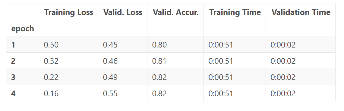
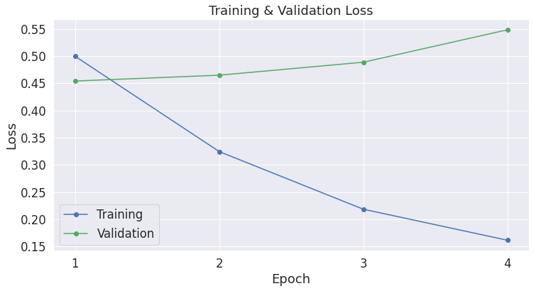
注意到,每次epoch,training loss都会降低,而validation loss却在上升!这意味着我们的训练模型的时间过长了,即模型过拟合了。validation loss 相对于准确率,是一个更精细的度量(measure),因为,对于准确率来说,我们并不关心实际的输出值,而是仅仅在乎输出值落在一个阈值的那一边。如果我们预测了正确的答案,但是这个预测的确信度比较低,那么validtaion loss将会捕捉到这一点,然而准确率却不能。
import matplotlib.pyplot as plt
% matplotlib inline

import seaborn as sns

# Use plot styling from seaborn.
sns.set(style='darkgrid')

# Increase the plot size and font size.
sns.set(font_scale=1.5)
plt.rcParams["figure.figsize"] = (12,6)

# Plot the learning curve.
plt.plot(df_stats['Training Loss'], 'b-o', label="Training")
plt.plot(df_stats['Valid. Loss'], 'g-o', label="Validation")

# Label the plot.
plt.title("Training & Validation Loss")
plt.xlabel("Epoch")
plt.ylabel("Loss")
plt.legend()
plt.xticks([1, 2, 3, 4])

plt.show()
5. Performance On Test Set
下面我们加载测试集,并使用 Matthew相关系数来评估模型性能,因为这是一种在 NLP 社区中被广泛使用的衡量 CoLA 任务性能的度量(metric)。使用这种测量方法,+1 为最高分,-1 为最低分。于是,我们就可以在特定任务上,横向和最好的模型进行性能对比了。
5.1. Data Preparation
我们将应用我们在训练集上做的相同的步骤,来准备我们的测试集数据。
import pandas as pd

# Load the dataset into a pandas dataframe.
df = pd.read_csv("./cola_public/raw/out_of_domain_dev.tsv", delimiter='\t', header=None, names=['sentence_source', 'label', 'label_notes', 'sentence'])

# Report the number of sentences.
print('Number of test sentences: {:,}\n'.format(df.shape[0]))

# Create sentence and label lists
sentences = df.sentence.values
labels = df.label.values

# Tokenize all of the sentences and map the tokens to thier word IDs.
input_ids = []
attention_masks = []

# For every sentence...
for sent in sentences:
    # `encode_plus` will:
    #   (1) Tokenize the sentence.
    #   (2) Prepend the `[CLS]` token to the start.
    #   (3) Append the `[SEP]` token to the end.
    #   (4) Map tokens to their IDs.
    #   (5) Pad or truncate the sentence to `max_length`
    #   (6) Create attention masks for [PAD] tokens.
    encoded_dict = tokenizer.encode_plus(
                        sent,                      # Sentence to encode.
                        add_special_tokens = True, # Add '[CLS]' and '[SEP]'
                        max_length = 64,           # Pad & truncate all sentences.
                        pad_to_max_length = True,
                        return_attention_mask = True,   # Construct attn. masks.
                        return_tensors = 'pt',     # Return pytorch tensors.
                   )

    # Add the encoded sentence to the list.
    input_ids.append(encoded_dict['input_ids'])

    # And its attention mask (simply differentiates padding from non-padding).
    attention_masks.append(encoded_dict['attention_mask'])

# Convert the lists into tensors.
input_ids = torch.cat(input_ids, dim=0)
attention_masks = torch.cat(attention_masks, dim=0)
labels = torch.tensor(labels)

# Set the batch size.
batch_size = 32

# Create the DataLoader.
prediction_data = TensorDataset(input_ids, attention_masks, labels)
prediction_sampler = SequentialSampler(prediction_data)
prediction_dataloader = DataLoader(prediction_data, sampler=prediction_sampler, batch_size=batch_size)
Number of test sentences: 516
5.2. Evaluate on Test Set
准备好测试集数据后,就可以用之前微调的模型来对测试集进行预测了.
# Prediction on test set

print('Predicting labels for {:,} test sentences...'.format(len(input_ids)))

# Put model in evaluation mode
model.eval()

# Tracking variables
predictions , true_labels = [], []

# Predict
for batch in prediction_dataloader:
  # Add batch to GPU
  batch = tuple(t.to(device) for t in batch)

  # Unpack the inputs from our dataloader
  b_input_ids, b_input_mask, b_labels = batch

  # Telling the model not to compute or store gradients, saving memory and
  # speeding up prediction
  with torch.no_grad():
      # Forward pass, calculate logit predictions
      outputs = model(b_input_ids, token_type_ids=None,
                      attention_mask=b_input_mask)

  logits = outputs[0]

  # Move logits and labels to CPU
  logits = logits.detach().cpu().numpy()
  label_ids = b_labels.to('cpu').numpy()

  # Store predictions and true labels
  predictions.append(logits)
  true_labels.append(label_ids)

print('    DONE.')
Predicting labels for 516 test sentences...
    DONE.
我们使用MCC,是因为类别是不平衡的。
print('Positive samples: %d of %d (%.2f%%)' % (df.label.sum(), len(df.label), (df.label.sum() / len(df.label) * 100.0)))
Positive samples: 354 of 516 (68.60%)
from sklearn.metrics import matthews_corrcoef

matthews_set = []

# Evaluate each test batch using Matthew's correlation coefficient
print('Calculating Matthews Corr. Coef. for each batch...')

# For each input batch...
for i in range(len(true_labels)):

  # The predictions for this batch are a 2-column ndarray (one column for "0"
  # and one column for "1"). Pick the label with the highest value and turn this
  # in to a list of 0s and 1s.
  pred_labels_i = np.argmax(predictions[i], axis=1).flatten()

  # Calculate and store the coef for this batch.
  matthews = matthews_corrcoef(true_labels[i], pred_labels_i)
  matthews_set.append(matthews)
Calculating Matthews Corr. Coef. for each batch...


/usr/local/lib/python3.6/dist-packages/sklearn/metrics/_classification.py:900: RuntimeWarning: invalid value encountered in double_scalars
  mcc = cov_ytyp / np.sqrt(cov_ytyt * cov_ypyp)
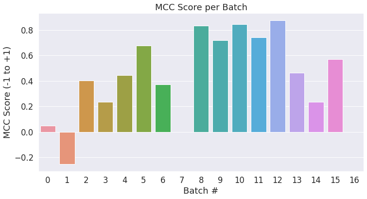
最终评测结果会基于整个的测试数据,不过我们可以统计每个小批量各自的分数,以查看批量之间的变化。
# Create a barplot showing the MCC score for each batch of test samples.
ax = sns.barplot(x=list(range(len(matthews_set))), y=matthews_set, ci=None)

plt.title('MCC Score per Batch')
plt.ylabel('MCC Score (-1 to +1)')
plt.xlabel('Batch #')

plt.show()
我们将所有批量的结果合并,来计算最终的 MCC 分数。
# Combine the results across all batches.
flat_predictions = np.concatenate(predictions, axis=0)

# For each sample, pick the label (0 or 1) with the higher score.
flat_predictions = np.argmax(flat_predictions, axis=1).flatten()

# Combine the correct labels for each batch into a single list.
flat_true_labels = np.concatenate(true_labels, axis=0)

# Calculate the MCC
mcc = matthews_corrcoef(flat_true_labels, flat_predictions)

print('Total MCC: %.3f' % mcc)
Total MCC: 0.498
Cool!只用了半个小时,在没有调整任何超参数的情况下(调整学习率、epochs、batch size、ADAM 属性等),我们却得到了一个不错的分数。
Note:为了最大化分数,我们应该移出validation set(我们使用它去帮助决定多少epochs去训练),然后再整个训练集上进行训练。
注意到(由于这个小的数据集大小),准确率会变化非常明显在我们运行时。
Conclusion
本教程展示了通过一个预训练BERT模型,你可以通过很小的努力和训练时间,在你感兴趣的特定的NLP任务上,快速和有效地创造一个高质量的模型。
Appendix
A1. Saving & Loading Fine-Tuned Model
下面的代码(源自 run_glue.py)将模型和分词器写到磁盘上。
import os

# Saving best-practices: if you use defaults names for the model, you can reload it using from_pretrained()

output_dir = './model_save/'

# Create output directory if needed
if not os.path.exists(output_dir):
    os.makedirs(output_dir)

print("Saving model to %s" % output_dir)

# Save a trained model, configuration and tokenizer using `save_pretrained()`.
# They can then be reloaded using `from_pretrained()`
model_to_save = model.module if hasattr(model, 'module') else model  # Take care of distributed/parallel training
model_to_save.save_pretrained(output_dir)
tokenizer.save_pretrained(output_dir)

# Good practice: save your training arguments together with the trained model
# torch.save(args, os.path.join(output_dir, 'training_args.bin'))
Saving model to ./model_save/


('./model_save/vocab.txt',
 './model_save/special_tokens_map.json',
 './model_save/added_tokens.json')
出于好奇心,让我们查看一下文件尺寸。
!ls -l --block-size=K ./model_save/
total 427960K
-rw-r--r-- 1 root root      2K Mar 18 15:53 config.json
-rw-r--r-- 1 root root 427719K Mar 18 15:53 pytorch_model.bin
-rw-r--r-- 1 root root      1K Mar 18 15:53 special_tokens_map.json
-rw-r--r-- 1 root root      1K Mar 18 15:53 tokenizer_config.json
-rw-r--r-- 1 root root    227K Mar 18 15:53 vocab.txt
最大的文件是模型权重,约418M左右。
!ls -l --block-size=M ./model_save/pytorch_model.bin
-rw-r--r-- 1 root root 418M Mar 18 15:53 ./model_save/pytorch_model.bin
将 Colab Notebook 中的模型存储到 Google Drive 上
# Mount Google Drive to this Notebook instance.
from google.colab import drive
    drive.mount('/content/drive')
# Copy the model files to a directory in your Google Drive.
!cp -r ./model_save/ "./drive/Shared drives/ChrisMcCormick.AI/Blog Posts/BERT Fine-Tuning/"
下面的函数将从磁盘上加载模型。
# Load a trained model and vocabulary that you have fine-tuned
model = model_class.from_pretrained(output_dir)
tokenizer = tokenizer_class.from_pretrained(output_dir)

# Copy the model to the GPU.
model.to(device)
A.2. Weight Decay
huggingface 的例子中包含以下代码来设置权重衰减(weight decay),但默认的衰减率为 "0",所以我把这部分代码移到了附录中。这个代码段本质上告诉优化器不在 bias 参数上运用权重衰减,权重衰减实际上是一种在计算梯度后的正则化,我们乘以它们,例如,0.99.
# This code is taken from:
# https://github.com/huggingface/transformers/blob/5bfcd0485ece086ebcbed2d008813037968a9e58/examples/run_glue.py#L102

# Don't apply weight decay to any parameters whose names include these tokens.
# (Here, the BERT doesn't have `gamma` or `beta` parameters, only `bias` terms)
no_decay = ['bias', 'LayerNorm.weight']

# Separate the `weight` parameters from the `bias` parameters.
# - For the `weight` parameters, this specifies a 'weight_decay_rate' of 0.01.
# - For the `bias` parameters, the 'weight_decay_rate' is 0.0.
optimizer_grouped_parameters = [
    # Filter for all parameters which *don't* include 'bias', 'gamma', 'beta'.
    {'params': [p for n, p in param_optimizer if not any(nd in n for nd in no_decay)],
     'weight_decay_rate': 0.1},

    # Filter for parameters which *do* include those.
    {'params': [p for n, p in param_optimizer if any(nd in n for nd in no_decay)],
     'weight_decay_rate': 0.0}
]

# Note - `optimizer_grouped_parameters` only includes the parameter values, not
# the names.
