【笔记】凸优化 Convex Optimization

Differentiation

Def. Gradient
$f:{\cal X}\sube\mathbb{R} ^N\to \mathbb{R}$ is differentiable. Then the gradient of $f$ at ${\bf x}\in\cal{X}$, denoted by $\nabla f({\bf x})$, is defined by

$$\nabla f({\bf x}) = \begin{bmatrix} \frac{\partial f}{\partial {\bf x} _1}({\bf x}) \\ \vdots \\ \frac{\partial f}{\partial {\bf x} _N}({\bf x}) \end{bmatrix}$$

Def. Hessian
$f:{\cal X}\sube\mathbb{R} ^N\to \mathbb{R}$ is twice differentiable. Then the Hessian of $f$ at ${\bf x}\in\cal{X}$, denoted by $\nabla ^2 f({\bf x})$, is defined by

$$\nabla ^2 f({\bf x}) = \begin{bmatrix} \frac{\partial ^2 f}{\partial {\bf x} _1^2}({\bf x}) & \cdots & \frac{\partial ^2 f}{\partial {\bf x} _1, {\bf x} _N}({\bf x}) \\ \vdots & \ddots & \vdots \\ \frac{\partial ^2 f}{\partial {\bf x} _N, {\bf x} _1}({\bf x}) & \cdots & \frac{\partial ^2 f}{\partial {\bf x} _N^2}({\bf x}) \end{bmatrix}$$

Th. Fermat's theorem
$f:{\cal X}\sube\mathbb{R} ^N\to \mathbb{R}$ is twice differentiable. If $f$ admits a local extrememum at ${\bf x} ^ *$, then $\nabla f(\bf x ^ *)=0$

Convexity

Def. Convex set
A set ${\cal X}\sube \mathbb{R} ^N$ is said to be convex, if for any ${\bf x, y}\in \cal X$, the segment $\bf [x, y]$ lies in $\cal X$, that is $\{\alpha{\bf x} + (1-\alpha){\bf y}:0\le\alpha\le 1 \}\sube\cal X$

Th. Operations that preserve convexity

• ${\cal C} _i$ is convex for all $i\in I$, then $\bigcap _{i\in I} {\cal C} _i$ is also convex
• ${\cal C} _1, {\cal C} _2$ is convex, then ${\cal C _1+C _2}=\{x _1+x _2:x _1\in {\cal C} _1, x _2\in {\cal X} _2 \}$ is also convex
• ${\cal C} _1, {\cal C} _2$ is convex, then ${\cal C _1\times C _2}=\{(x _1, x _2):x _1\in {\cal C} _1, x _2\in {\cal X} _2 \}$ is also convex
• Any projection of a convex set is also convex

Def. Convex hull
The Convex hull $\text{conv}(\cal X)$ of set ${\cal X}\sube \mathbb{R} ^N$, is the minimal convex set containing $\cal X$, that is

$$\text{conv}({\cal X})=\left\{ \sum _{i=1}^m \alpha _i {\bf x} _i:\forall ({\bf x} _1,\dotsb, {\bf x} _m)\in {\cal X}, \alpha _i\ge 0, \sum _{i=1} ^m \alpha _i = 1 \right\}$$

Def. Epigraph
The epigraph of $f:{\cal X}\to \mathbb{R}$, denoted by $\text{Epi } f$, is defined by $\{(x,y):x\in {\cal X}, y\ge f(x)\}$

Def. Convex function
Convex set $\cal X$. A function $f:{\cal X}\to \mathbb{R}$ is said to be convex, iff $\text{Epi }f$ is convex, or equivalently, for all ${\bf x, y}\in {\cal X},\alpha \in [0,1]$

$$f(\alpha{\bf x} + (1-\alpha){\bf y})\le \alpha f({\bf x}) + (1-\alpha) f({\bf y})$$

Moreover, $f$ is said to be strictly convex if the inequality is strict when $\bf x\ne y$ and $\alpha\in (0,1)$. $f$ is said to be (strictly) concave if $-f$ is (strictly) convex.

Th. Convex function characterized by first-order differential
$f:{\cal X}\sube\mathbb{R} ^N\to \mathbb{R}$ is differentiable. Then $f$ is convex iff $\text{dom}(f)$ is convex, and

$$\forall {\bf x, y}\in \text{dom}(f),\quad f({\bf y})-f({\bf x})\ge \nabla f({\bf x})\cdot({\bf y-x})$$

交换 $\bf x, y$，得到 $f({\bf x})-f({\bf y})\ge \nabla f({\bf y})\cdot({\bf x-y})$，相加得：

$$\lang\nabla f({\bf x}) - \nabla f({\bf y}),{\bf x-y}\rang\ge 0$$

其含义为 “梯度单调且内积大等于零”，这也是凸性的等价条件之一

Th. Convex function characterized by second-order differential
$f:{\cal X}\sube\mathbb{R} ^N\to \mathbb{R}$ is twice differentiable. Then $f$ is convex iff $\text{dom}(f)$ is convex, and its Hessian is positive semidefinite (半正定)

$$\forall {\bf x}\in \text{dom}(f),\quad \nabla ^2 f({\bf x})\succeq 0$$

• 对称阵为半正定，若其所有特征值非负；$A\succeq B$ 等价于 $A-B$ 为半正定
• If $f$ is scalar (eg. $x\mapsto x ^2$), then $f$ is convex iff $\forall x\in \text{dom}(f), f''(x)\ge 0$
• For example
  • Linear functions is both convex and concave
  • Any norm $\Vert\cdot\Vert$ over convex set $\cal X$ is a convex function
    $\Vert\alpha{\bf x}+(1-\alpha){\bf y} \Vert\le \Vert\alpha{\bf x}\Vert+\Vert(1-\alpha){\bf y} \Vert\le \alpha\Vert{\bf x}\Vert+(1-\alpha)\Vert{\bf y}\Vert$
• Using composition rules to prove convexity

Th. Composition of convex/concave functions
Assume $h:\mathbb{R}\to\mathbb{R}$ and $g:\mathbb{R} ^N\to\mathbb{R}$ are twice differentiable. Define $f({\bf x})=h(g({\bf x})), \forall {\bf x}\in \mathbb{R} ^N$, then

• $h$ is convex & non-decreasing, $g$ is convex $\implies$ $f$ is convex
• $h$ is convex & non-increasing, $g$ is concave $\implies$ $f$ is convex
• $h$ is concave & non-decreasing, $g$ is concave $\implies$ $f$ is concave
• $h$ is concave & non-increasing, $g$ is convex $\implies$ $f$ is concave

Proof: It holds for $N=1$, which suffices to prove convexity (concavity) along all lines that intersect the domain.
Example: $g$ could be any norm $\Vert\cdot\Vert$

Th. Pointwise maximum of convex functions
$f _i$ is a convex function defined over convex set $\cal C$ for all $i\in I$, then $f(x)=\sup _{i\in I}f _i(x), x\in \cal C$ is a convex function.
Proof: $\text{Epi } f = \bigcap _{i\in I} \text{Epi } f _i$ is convex

• $f({\bf x})=\max _{i\in I}{\bf w} _i\cdot {\bf x}+b _i$ over a convex set, is a convex function
• The maximum eigenvalue $\lambda _{\max}({\bf M})$ over the set of symmetric matrices, is a convex function, since $\lambda _{\max}({\bf M})=\sup _{\Vert\bf x\Vert _2\le 1}{\bf x}'{\bf Mx}$ is supremum of linear functions ${\bf M}\mapsto{\bf x}'{\bf Mx}$
  More generally, let $\lambda _{k}(\bf M)$ denote the top $k$ eigenvalues, then ${\bf M}\mapsto \sum _{i=1} ^{k}\lambda _{i}(\bf M)$ and ${\bf M}\mapsto \sum _{i=n-k+1} ^{n}\lambda _{i}({\bf M})=-\sum _{i=1} ^{k}\lambda _i(-\bf M)$ are both convex function

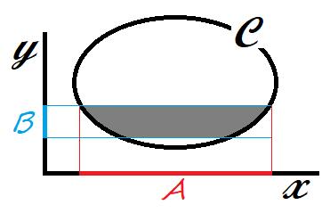
Th. Partial infimum
Convex function $f$ defined over convex set $\cal C\sube X\times Y$, and conves set $\cal B\sube Y$. Then ${\cal A}=\{x\in {\cal X}:\exist y\in{\cal B}, (x, y)\in {\cal C} \}$ is convex set if non-empty, and $g(x)=\inf _{y\in\cal B} f(x, y)$ for all $x\in \cal A$ is convex function.
For example, the distance to convex set $\cal B$, $d(x)=\inf _{y\in \cal B}\Vert x-y\Vert$ is convex function

Th. Jensen's inequality
Let r.v. $X$ in convex set ${\cal C}\sube \mathbb{R} ^N$, and convex function $f$ defined over $\cal C$. Then, $\mathbb{E}[X]\in {\cal C}, \mathbb{E}[f(X)]$ is finite, and

$$f(\mathbb{E}[X])\le \mathbb{E}[f(X)]$$

Sketch of proof: extending $f(\sum \alpha x)\le\sum \alpha f(x)$ and $\sum \alpha=1$ that can be interpreted as probabilities, to arbitraty contributions.

Smoothness, strong convexity

参考 [https://zhuanlan.zhihu.com/p/619288199]
考虑二阶导的 lipschitz 连续性

Def. $\beta$-smooth
称函数 $f$ 是 $\beta$-smooth 的，若

$$\forall{\bf x, y}\in\text{dom}(f),\quad \Vert\nabla f({\bf x}) - \nabla f({\bf y})\Vert\le \beta\Vert {\bf x-y}\Vert$$

等价于如下命题均成立：

• $\frac{\beta}{2}\Vert {\bf x}\Vert ^2 - f({\bf x})$ 是凸函数
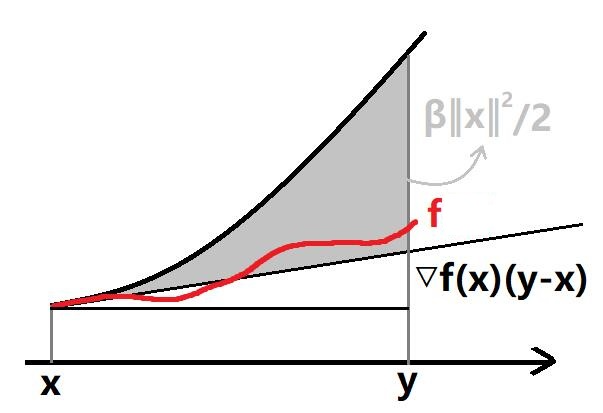
• $\forall{\bf x, y}\in\text{dom}(f),\quad f({\bf y})\le f({\bf x}) + \nabla f({\bf x}) ^\top ({\bf y-x}) + \frac{\beta}{2} \Vert{\bf y-x}\Vert ^2$
• $\nabla ^2 f({\bf x})\preceq \beta I$

证明/说明
证明 $g({\bf x})=\frac{\beta}{2}\Vert {\bf x}\Vert ^2 - f({\bf x})$ 为凸，可以考虑 $\lang\nabla g({\bf x}) - \nabla g({\bf y}),{\bf x-y}\rang\ge 0$，应用柯西不等式可证
感性理解之，$f$ 的起伏 “拗不过” $\frac{\beta}{2}\Vert {\bf x}\Vert ^2$ 的凸性，即 $f$ 起伏不够大，也就是比较平滑 smooth
证明第二、三条，代入 $g({\bf y})-g({\bf x})\ge \nabla g({\bf x})\cdot({\bf y-x})$ 和 $\nabla ^2 g({\bf x})\succeq 0$ 即可；它的几何含义见下

Def. $\alpha$-strongly convex
称函数 $f$ 是 $\alpha$-strongly convex 的，若

• $\forall{\bf x, y}\in\text{dom}(f),\quad \Vert\nabla f({\bf x}) - \nabla f({\bf y})\Vert\ge \alpha\Vert {\bf x-y}\Vert$
• $f({\bf x}) - \frac{\alpha}{2}\Vert {\bf x}\Vert ^2$ 是凸函数
• $\forall{\bf x, y}\in\text{dom}(f),\quad f({\bf y})\ge f({\bf x}) + \nabla f({\bf x}) ^\top ({\bf y-x}) + \frac{\alpha}{2} \Vert{\bf y-x}\Vert ^2$
• $\nabla ^2 f({\bf x})\succeq \alpha I$

Def. $\gamma$-well-conditioned
称函数 $f$ 是 $\gamma$-well-conditioned 的，若其同时是 $\alpha$-strongly convex 和 $\beta$-smooth 的；定义 $f$ 的 condition number 为 $\gamma=\alpha /\beta\le 1$

Th. Linear combination of two convex functions

• 考虑两个凸函数的加和，有：
  • 若 $f$ 为 $\alpha _1$-strongly convex，$g$ 为 $\alpha _2$-strongly convex，则 $f+g$ 为 $(\alpha _1+\alpha _2)$-strongly convex
  • 若 $f$ 为 $\beta _1$-smooth，$g$ 为 $\beta _2$-smooth，则 $f+g$ 为 $(\beta _1 + \beta _2)$-smooth
• 考虑凸函数的数乘 $k>0$，有：
  • 若 $f$ 为 $\alpha$-strongly convex，则 $kf$ 为 $(k\alpha)$-strongly convex
  • 若 $f$ 为 $\beta$-smooth，则 $kf$ 为 $(k\beta)$-smooth

证明，利用凸函数满足 $\lang\nabla f({\bf x}) - \nabla f({\bf y}),{\bf x-y}\rang\ge 0$ 和 $\frac{\beta}{2}\Vert {\bf x}\Vert ^2 - f({\bf x}), f({\bf x}) - \frac{\alpha}{2}\Vert {\bf x}\Vert ^2$ 的凸性即可

Projections onto convex sets

之后的算法会涉及向凸集投影的概念；定义 $\bf y$ 向凸集 $\cal K$ 的投影，为

$$\prod _{\cal K}({\bf y})\triangleq \underset{{\bf x}\in\cal K}{\text{arg min }} \Vert {\bf x-y}\Vert$$

可以证明投影总是唯一的；投影还具有一个很重要的性质：
Th. Pythagorean theorem 勾股定理
凸集 $\cal K\sube \mathbb{R} ^d,{\bf y}\in\mathbb{R} ^d,{\bf x}=\prod _{\cal K}({\bf y})$，则任意 $\bf z\in\cal K$，$\bf \Vert y-z\Vert\ge \Vert x-z\Vert$
即，对凸集内的任一点，其到投影点的距离不大于其到被投影点的距离

Constrained optimization 带约束优化

Def. Constrained optimization problem
${\cal X}\sube \mathbb{R} ^N,\ f, g _i:{\cal X}\to\mathbb{R}, i\in [m]$，则带约束优化问题（也称为 primal problem）的形式为

$$\min _{\bf x\in\cal X} f({\bf x}) \\ subject\ to: g _i({\bf x})\le 0, \forall i\in [m]$$

记 $\inf _{\bf x\in\cal X} f({\bf x})=p ^ *$；注意到目前我们没有假设任何的 convexity；对于 $g=0$ 的约束我们可以用 $g\le 0, -g\le 0$ 来刻画

Dual problem and saddle point

解决这类问题，可以先引入拉格朗日函数 Lagrange function，将约束以非正项引入；然后转化成对偶问题

Def. Lagrange function
为带约束优化问题定义拉格朗日函数，为

$$\forall {\bf x}\in {\cal X},\forall{\boldsymbol{\alpha}\ge 0},\quad {\cal L}({\bf x}, {\boldsymbol{\alpha}})=f({\bf x}) + \sum _{i=1}^{m} \alpha _i g _i({\bf x})$$

其中 ${\boldsymbol{\alpha}}=(\alpha _1,\dotsb, \alpha _m)'$ 称为对偶变量 dual variable
对于约束 $g=0$，其系数 $\alpha=\alpha _+ - \alpha _-$ 不需要非负（但是下文给出定理时，要求 $g,-g$ 同时为凸，从而 $g$ 得是仿射函数 affine，即形如 ${\bf w\cdot x+b}$）
注意到 $p ^ * = \inf _{\bf x} \sup _{\boldsymbol{\alpha}}{\cal L}({\bf x}, {\boldsymbol{\alpha}})$，因为当 $\bf x$ 不满足约束时 $\sup _{\boldsymbol{\alpha}}$ 可以取到无穷大，从而刻画了约束
有趣的来了，我们能构造一个 concave function，称为对偶函数 Dual function

Def. Dual function
为带约束优化问题定义对偶函数，为

$$\forall{\boldsymbol{\alpha}}\ge 0,\quad F({\boldsymbol{\alpha}})=\inf _{\bf x\in\cal X} {\cal L}({\bf x},{\boldsymbol{\alpha}})=\inf _{\bf x\in\cal X} \left(f({\bf x}) + \sum _{i=1}^{m} \alpha _i g _i({\bf x})\right)$$

它是 concave 的，因为 $\cal L$ 是关于 $\boldsymbol{\alpha}$ 的线性函数，且 pointwise infimum 保持了 concavity
同时注意到对任意 ${\boldsymbol{\alpha}}$，$F({\boldsymbol{\alpha}})\le \inf _{\bf x\in\cal X}f({\bf x})=p ^ *$
定义对偶问题

Def. Dual problem
为带约束优化问题定义对偶问题，为

$$\max _{\boldsymbol{\alpha}} F({\boldsymbol{\alpha}}) \\ subject\ to:{\boldsymbol{\alpha}}\ge 0$$

对偶问题是凸优化问题，即求 concave 函数的最大值，记其为 $d ^ *$；由上文可知 $d ^ *\le p ^ *$，也就是：

$$d ^ * = \sup _{\boldsymbol{\alpha}} \inf _{\bf x} {\cal L}({\bf x}, {\boldsymbol{\alpha}})\le \inf _{\bf x} \sup _{\boldsymbol{\alpha}}{\cal L}({\bf x}, {\boldsymbol{\alpha}}) = p ^ *$$

称为弱对偶 weak duality，取等情况称为强对偶 strong duality
接下来会给出：

当凸优化问题满足约束规范性条件 constraint qualification (Slater's contidion) 时（此为充分条件），有 $d ^ *=p ^ *$，且该解的充要条件为拉格朗日函数的鞍点 saddle point

Def. Constraint qualification (Slater's condition)
假设集合 $\cal X$ 的内点非空 $\text{int}({\cal X})\ne \empty$：

• 定义 strong constraint qualification (Slater's condition) 为

$$\exist \bar{{\bf x}}\in\text{int}({\cal X}):\forall i\in [m], g _i(\bar{{\bf x}})< 0$$

• 定义 weak constraint qualification (weak Slater's condition) 为

$$\exist \bar{{\bf x}}\in\text{int}({\cal X}):\forall i\in [m], (g _i(\bar{{\bf x}})< 0)\vee (g _i(\bar{{\bf x}})=0\wedge g _i \text{ affine})$$

（这个条件是在说明解存在吗？）
基于 Slater's condition，叙述拉格朗日函数的鞍点 saddle point 是带约束优化问题的解的充要条件

Th. Saddle point - sufficient condition
带约束优化问题，如果其拉格朗日函数存在鞍点 saddle point $({\bf x} ^ *, \boldsymbol{\alpha} ^ *)$，即

$$\forall {\bf x}\in {\cal X},\forall{\boldsymbol{\alpha}\ge 0},\quad {\cal L}({\bf x} ^ *, {\boldsymbol{\alpha}})\le {\cal L}({\bf x} ^ *, {\boldsymbol{\alpha}} ^ *)\le {\cal L}({\bf x}, {\boldsymbol{\alpha}} ^ *)$$

则 ${\bf x} ^ *$ 是该问题的解，$f({\bf x} ^ *)=\inf f({\bf x})$

Th. Saddle point - necessary condition
假设 $f, g _i, i\in [m]$ 为 convex function：

• 若满足 Slater's condition，则带约束优化问题的解 $\bf x ^ *$ 满足存在 $\boldsymbol{\alpha} ^ *\ge 0$ 使得 $({\bf x} ^ *, \boldsymbol{\alpha} ^ *)$ 是拉格朗日函数的鞍点
• 若满足 weak Slater's condition 且 $f, g _i$ 可导，则带约束优化问题的解 $\bf x ^ *$ 满足存在 $\boldsymbol{\alpha} ^ *\ge 0$ 使得 $({\bf x} ^ *, \boldsymbol{\alpha} ^ *)$ 是拉格朗日函数的鞍点

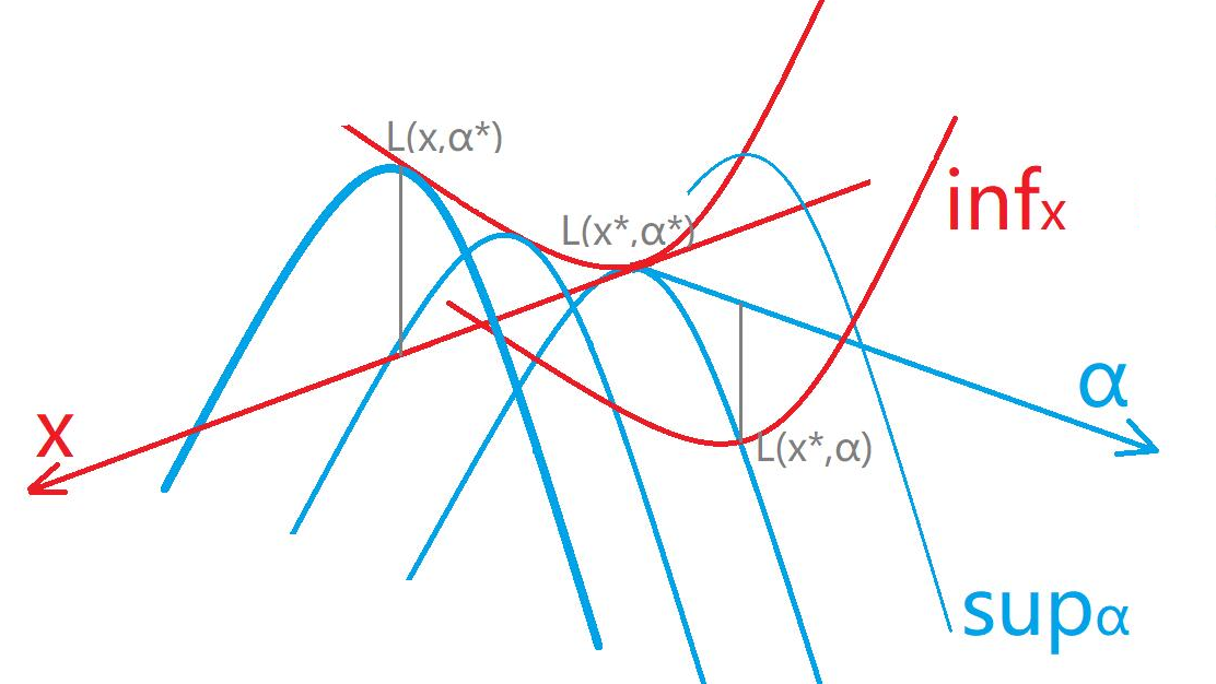
由于书本上没提供必要性的证明，且充分性证明不难但是不够漂亮，所以就不抄了，只给出我自己的思路（虽然可能有缺陷，下图也只是示意）：

回到最初的不等式：

$$d ^ * = \sup _{\boldsymbol{\alpha}} \inf _{\bf x} {\cal L}({\bf x}, {\boldsymbol{\alpha}})\le\inf _{\bf x} \sup _{\boldsymbol{\alpha}}{\cal L}({\bf x}, {\boldsymbol{\alpha}}) = p ^ *$$

定义 ${\bf x} ^ *$ 取到 $p ^ *=\sup _{\boldsymbol{\alpha}}{\cal L}({\bf x} ^ *, {\boldsymbol{\alpha}})\le \sup _{\boldsymbol{\alpha}}{\cal L}({\bf x}, {\boldsymbol{\alpha}}),\ \forall {\bf x}$（可能有多个）
定义 ${\boldsymbol{\alpha}} ^ *$ 取到 $d ^ *=\inf _{\bf x} {\cal L}({\bf x}, {\boldsymbol{\alpha} ^ *})\ge \inf _{\bf x} {\cal L}({\bf x}, {\boldsymbol{\alpha}}),\ \forall {\boldsymbol{\alpha}}$（可能有多个）
（鞍点）唯一性和函数凸性有关（虽然感觉不严格凸的话可以是一片“平”的区域），留给之后再说吧
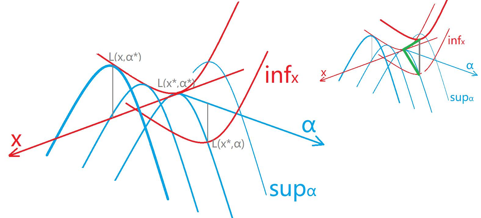
试证明：

$\cal L$ 存在鞍点、存在一组 $({\bf x} ^ *, {\boldsymbol{\alpha}} ^ *)$ 是鞍点、$p ^ * = d ^ *$、$p ^ * = d ^ * ={\cal L}({\bf x} ^ *, {\boldsymbol{\alpha}} ^ *)$ 四者等价

分别记为命题 $A,B,C,D$，显然有 $B\to A, D\to C$

证明 $A\to B, B\to CD$：
若存在鞍点（思路见图右上），记鞍点为 $({\bf x}' , {\boldsymbol{\alpha}}')$，则 ${\cal L}({\bf x}', {\boldsymbol{\alpha}} ^ *){\color{green}\le} {\cal L}({\bf x}', {\boldsymbol{\alpha}}')=\inf _{\bf x}{\cal L}({\bf x}, {\boldsymbol{\alpha}}'){\color{green}\le} \inf _{\bf x} {\cal L}({\bf x}, {\boldsymbol{\alpha} ^ *})$，观察不等式两头则取等；进而有 $\inf _{\bf x}{\cal L}({\bf x}, {\boldsymbol{\alpha}} ^ *)\le {\cal L}({\bf x}', {\boldsymbol{\alpha}} ^ *)= \inf _{\bf x}{\cal L}({\bf x}, {\boldsymbol{\alpha}}')$，根据 $\boldsymbol{\alpha} ^ *$ 定义该不等式取等，于是可以令 $\boldsymbol{\alpha} ^ *\leftarrow\boldsymbol{\alpha}'$；接下来对 $\bf x ^ *,x'$ 同理
此时 $({\bf x} ^ * , {\boldsymbol{\alpha}} ^ *)$ 是鞍点，即 $\forall {\bf x},\forall {\boldsymbol{\alpha}},\ {\cal L}({\bf x} ^ *, {\boldsymbol{\alpha}})\le {\cal L}({\bf x} ^ *, {\boldsymbol{\alpha}} ^ *)\le {\cal L}({\bf x}, {\boldsymbol{\alpha}} ^ *)$，则有 $p ^ * = \sup _{\boldsymbol{\alpha}}{\cal L}({\bf x} ^ *, {\boldsymbol{\alpha}}) = {\cal L}({\bf x} ^ *, {\boldsymbol{\alpha}} ^ *) = \inf _{\bf x} {\cal L}({\bf x}, {\boldsymbol{\alpha} ^ *}) = d ^ *$

证明 $C\to BD$：
若 $p ^ * =d ^ *$，即 $\sup _{\boldsymbol{\alpha}}{\cal L}({\bf x} ^ *, {\boldsymbol{\alpha}})=\inf _{\bf x} {\cal L}({\bf x}, {\boldsymbol{\alpha} ^ *})$，且 $\sup _{\boldsymbol{\alpha}}{\cal L}({\bf x} ^ *, {\boldsymbol{\alpha}})\ge {\cal L}({\bf x} ^ *, {\boldsymbol{\alpha} ^ *})\ge \inf _{\bf x} {\cal L}({\bf x}, {\boldsymbol{\alpha} ^ *})$；故三者取等，故 $\forall {\bf x},\forall {\boldsymbol{\alpha}},\ {\cal L}({\bf x} ^ *, {\boldsymbol{\alpha}})\le \sup _{\boldsymbol{\alpha}}{\cal L}({\bf x} ^ *, {\boldsymbol{\alpha}})={\cal L}({\bf x} ^ *, {\boldsymbol{\alpha} ^ *})=\inf _{\bf x} {\cal L}({\bf x}, {\boldsymbol{\alpha} ^ *})\le {\cal L}({\bf x}, {\boldsymbol{\alpha} ^ *})$，从而 $({\bf x} ^ * , {\boldsymbol{\alpha}} ^ *)$ 是鞍点

综上得证。爽！

KKT conditions

Lagrangian version

若带约束优化问题满足 convexity，我们就可以用一个定理解决：KKT

Th. Karush-Kuhn-Tucker's theorem
假设 $f, g _i:{\cal X}\to\mathbb{R},\forall i\in[m]$，为 convex and differentiable，且满足 Slater's condition；则带约束优化问题

$$\min _{\bf x\in\cal X, {\bf g}({\bf x})\le {\bf 0}} f({\bf x})$$

其拉格朗日函数为 ${\cal L}({\bf x}, {\boldsymbol{\alpha}})=f({\bf x}) + {\boldsymbol{\alpha}}\cdot {\bf g}({\bf x}), {\boldsymbol{\alpha}}\ge 0$
则 $\bar{\bf x}$ 是该问题的解，当且仅当存在 $\bar{\boldsymbol{\alpha}}\ge 0$，满足：

$$\begin{aligned} \nabla _{\bf x} {\cal L}(\bar{\bf x}, \bar{\boldsymbol{\alpha}}) &= \nabla _{\bf x} f(\bar{\bf x}) + \bar{\boldsymbol{\alpha}}\cdot \nabla _{\bf x} {\bf g}(\bar{\bf x}) = 0 \\ \nabla _{\boldsymbol{\alpha}} {\cal L}(\bar{\bf x}, \bar{\boldsymbol{\alpha}})&={\bf g}(\bar{\bf x})\le 0 \\ \bar{\boldsymbol{\alpha}}\cdot {\bf g}(\bar{\bf x}) &= 0 \end{aligned}\quad ;\text{KKT conditions}$$

其中后两条称为互补条件 complementarity conditions，即对任意 $i\in[m], \bar{\boldsymbol{\alpha}} _i\ge 0,g _i(\bar{\bf x})\le 0$，且满足 $\bar{\boldsymbol{\alpha}} _i g _i(\bar{\bf x})=0$

充要性证明：

必要性，$\bar{\bf x}$ 为解，则存在 $\bar{\boldsymbol{\alpha}}$ 使得 $(\bar{\bf x}, \bar{\boldsymbol{\alpha}})$ 为鞍点，从而得到 KKT 条件：第一条即鞍点定义，第二、三条：

$$\begin{aligned} \forall {{\boldsymbol{\alpha}}},{\cal L}(\bar{\bf x}, {\boldsymbol{\alpha}})\le{\cal L}(\bar{\bf x}, \bar{\boldsymbol{\alpha}})&\implies{\boldsymbol{\alpha}}\cdot {\bf g}(\bar{\bf x})\le \bar{\boldsymbol{\alpha}}\cdot {\bf g}(\bar{\bf x})\\{\boldsymbol{\alpha}}\to +\infty&\implies {\bf g}(\bar{\bf x})\le 0 \\ {\boldsymbol{\alpha}}\to 0 &\implies \bar{\boldsymbol{\alpha}}\cdot{\bf g}(\bar{\bf x})=0 \end{aligned}$$

充分性，满足 KKT 条件，则对于满足 $\bf g({\bf x})\le 0$ 的 $\bf x$：

$$\begin{aligned} f({\bf x}) - f(\bar{\bf x}) &\ge \nabla _{\bf x} f(\bar{\bf x})\cdot ({\bf x-\bar{x}}) & ;\text{convexity of $f$} \\ &= -\bar{\boldsymbol{\alpha}}\cdot \nabla _{\bf x} {\bf g}(\bar{\bf x})\cdot ({\bf x-\bar{x}}) &; \text{first cond}\\ &\ge -\bar{\boldsymbol{\alpha}}\cdot ({\bf g}({\bf x})-{\bf g}(\bar{\bf x})) &; \text{convexity of $g$}\\ &= -\bar{\boldsymbol{\alpha}}\cdot {\bf g}({\bf x}) \ge 0 &;\text{third cond} \end{aligned}$$

Gradient descent version

我们还能用另一种思路阐述 KKT 定理，并且也是另一种求解带约束优化问题的方法：梯度下降
由于 $\bf g$ 均为凸函数，显然 ${\cal K}=\{\bf x:g(x)\le 0\}$ 为凸集；因此约束其实就是把取值限定在凸集 $\cal K$ 上，于是有：

Th. Karush-Kuhn-Tucker's theorem, gradient descent version
假设 $f$ 为 convex and differentiable，$\cal K$ 为凸集；则带约束优化问题

$$\min _{\bf x\in\cal K} f({\bf x})$$

则 $\bf x ^ *$ 是该问题的解，当且仅当

$$\forall {\bf y}\in{\cal K},\quad -\nabla f({\bf x ^ *}) ^\top ({\bf y-x ^ *}) \le 0$$

其思想为，负梯度方向为 $f$ 函数值下降的方向，若其与 $\bf y-x ^ *$ 有相同方向的分量（内积大于零），则可以沿该方向移动，则 $\bf x ^ *$ 不会是最优点
这个定理为我们的梯度下降算法提供了基础

Gradient descent

Unconstrained case

无约束凸优化问题的梯度下降 GD 算法
记 $\nabla _t=\nabla f({\bf x} _t),h _t=f({\bf x} _t)-f({\bf x} ^ *),d _t = \Vert{\bf x} _t-{\bf x} ^ * \Vert$

$$\begin{aligned} \hline & \underline{\text{Algorithm. Gradient descent}\qquad\qquad\qquad\qquad\qquad} \\ & \text{Input $T, {\bf x} _0, \{\eta _t\}$} \\ & \text{for $t=0,\dotsb, T-1$ do} \\ & \qquad \text{${\bf x} _{t+1} = {\bf x} _t - \eta _t \nabla _t$} \\ & \text{end for} \\ & \text{return $\bar{\bf x}=\text{argmin} _{{\bf x} _t}\{ f({\bf x} _t) \}$} \\ \hline \end{aligned}$$

其中合理地选择 $\eta _t$，决定了算法的效率；取 Polyak stepsize：$\eta _t=\frac{h _t}{\Vert \nabla _t\Vert ^2}$，有：

Th. Bound for GD with Polyak stepsize
假设 $\Vert \nabla _t\Vert\le G$，则

$$f(\bar{\bf x}) - f({\bf x} ^ *)=\min _{0\le t\le T}\{h _t\}\le \min \left\{ \frac{G d _0}{\sqrt{T}},\frac{2\beta d _0 ^2}{T}, \frac{3G ^2}{\alpha T},\beta d _0 ^2(1-\frac{\gamma}{4}) ^T \right\}$$

该定理的证明建立在 $d _{t+1} ^2\le d _t ^2 - {h _t ^2}/{\Vert \nabla _t\Vert ^2}$ 上，这就感觉很扯淡了，因为用绝对值不等式放缩出来总是反的...
证明算法的效率时，可以用一些 “potential 势差” 函数来刻画，比如刻画势能 $h _t = f({\bf x} _t)-f({\bf x} ^ *)$ 的降低，考虑势能差 $h _{t+1}-h _t$、梯度的范数 $\Vert\nabla _t\Vert$；比如到最优点的距离 $d _t = \Vert {\bf x-x} ^ *\Vert$ 的降低，考虑 $d _{t+1}-d _t$；
先给出引理，代入 smooth 和 strong convexity 可以证明；这些式子方便我们后续进行放缩

$$\frac{\alpha}{2}d _t ^2\le h _t\le \frac{\beta}{2}d _t ^2\\ \frac{1}{2\beta}\Vert \nabla _t \Vert ^2\le h _t\le \frac{1}{2\alpha}\Vert \nabla _t \Vert ^2$$

对于更新式 ${\bf x} _{t+1} = {\bf x} _t - \eta _t \nabla _t$，如果考虑 $d _{t+1}-d _t$，那就两边同减 $\bf x ^ *$ 并取范数，用三角不等式放缩，但是符号和上文的假设是反的，到此就证不下去了；如果假定 $d _{t+1} ^2\le d _t ^2 - {h _t ^2}/{\Vert \nabla _t\Vert ^2}$，那就能证明上面的 bound（注意 $f(\bar{\bf x})-f({\bf x} ^ * )\le \frac{1}{T}\sum _t h _t$ 可以不等式放缩）
不过，我们可以从 $h _{t+1}-h _t$ 出发，有：

$$\begin{aligned}h _{t+1}-h _t &= f({\bf x} _{t+1})-f({\bf x} _{t})\\ &\le \nabla f({\bf x} _t) ^\top({\bf x} _{t+1} - {\bf x} _{t})+\frac{\beta}{2}\Vert {\bf x} _{t+1}-{\bf x} _{t}\Vert ^2 \\ &= -\eta _t\Vert \nabla _t\Vert ^2+\frac{\beta}{2}\eta _t ^2\Vert \nabla _t\Vert ^2\\ &=-\frac{1}{2\beta}\Vert \nabla _t \Vert ^2\qquad ;\text{令 }\eta _t=\frac{1}{\beta} \\ &\le -\frac{\alpha}{\beta}h _t=-\gamma h _t\end{aligned}$$

于是 $h _{T}\le (1-\gamma) h _{T-1}\le (1-\gamma) ^T h _0\le e ^{-\gamma T} h _0$，这倒是个很不错的收敛保证，因此有

Th. Bound for GD, unconstrained case
假设 $f$ 是 $\gamma$-well-conditioned，令 $\eta _t=\frac{1}{\beta}$，则

$$h _{T}\le e ^{-\gamma T} h _0$$

Constrained case

带约束优化的梯度下降，只需要每次移动后，投影到凸集

$$\begin{aligned} \hline & \underline{\text{Algorithm. Basic gradient descent}\qquad\qquad\qquad\qquad\qquad} \\ & \text{Input $T, {\bf x} _0\in{\cal K}, \{\eta _t\}$} \\ & \text{for $t=0,\dotsb, T-1$ do} \\ & \qquad {\bf x} _{t+1} = \Pi _{\cal K}({\bf x} _t - \eta _t \nabla _t) \\ & \text{end for} \\ & \text{return $\bar{\bf x}=\text{argmin} _{{\bf x} _t}\{ f({\bf x} _t) \}$} \\ \hline \end{aligned}$$

它有个类似的上限：
Th. Bound for GD, constrained case
假设 $f$ 是 $\gamma$-well-conditioned，令 $\eta _t=\frac{1}{\beta}$，则

$$h _{T}\le e ^{-\gamma T/4} h _0$$

证明
首先是投影的定义

$$\begin{aligned} {\bf x} _{t+1} &= \Pi _{\cal K}({\bf x} _t - \eta _t \nabla _t) \\ &= \text{argmin} _{\bf x} \Vert {\bf x} - {\bf x} _t + \eta _t \nabla _t \Vert \\ &= \text{argmin} _{\bf x}( \nabla _t ^\top ({\bf x - x} _t) + \frac{1}{2\eta _t}\Vert {\bf x - x} _t\Vert ^2 ) \end{aligned}$$

根据如下式子，可以令 $\eta _t=\frac{1}{\beta}$；从而有：

$$\begin{aligned} h _{t+1}-h _t &= f ({\bf x} _{t+1}) - f ({\bf x} _t) \\ &\le \nabla _t ^\top ({\bf x} _{t+1} - {\bf x} _t) + \frac{\beta}{2}\Vert {\bf x} _{t+1} - {\bf x} _t\Vert ^2 \\ &= \text{min} _{\bf x} (\nabla _t ^\top ({\bf x} - {\bf x} _t) + \frac{\beta}{2}\Vert {\bf x} - {\bf x} _t\Vert ^2) \end{aligned}$$

为了摘掉 $\min$，我们可以代入某个 $\bf x$，代入哪个呢？可以考虑两点的连线，即 $(1-\mu){\bf x} _t + \mu {\bf x} ^ *$：

$$\begin{aligned} h _{t+1}-h _t &\le \text{min} _{\bf x\in [{\bf x} _t, {\bf x} ^ * ]} (\nabla _t ^\top ({\bf x} - {\bf x} _t) + \frac{\beta}{2}\Vert {\bf x} - {\bf x} _t\Vert ^2) \\ &\le \mu \nabla _t ^\top ({\bf x} ^ * - {\bf x} _t) +\mu ^2 \frac{\beta}{2}\Vert {\bf x} ^ * - {\bf x} _t \Vert ^2 \\ &\le -\mu h _t + \mu ^2 \frac{\beta-\alpha}{2}\Vert {\bf x} ^ * - {\bf x} _t \Vert ^2\quad; \alpha\text{-strong convex}\\ &\le -\mu h _t + \mu ^2\frac{\beta - \alpha}{\alpha}h _t \quad;\text{Lemma} \end{aligned}$$

对 $\mu\in[0,1]$ 取极值，得到

$$h _{t+1}\le h _t(1-\frac{\alpha}{4(\beta-\alpha)})\le h _t(1-\frac{\gamma}{4})\le h _t e ^{-\gamma/4}$$

从而得证

GD: Reductions to non-smooth and non-strongly convex functions

现在来考虑梯度下降对不一定 smooth、或不一定 strong convex 的凸函数时该怎么分析；下文提到的 reduction 方法可以导出近似最优的收敛速度，而且很简单、很普适

Case 1. reduction to smooth, non-strongly convex functions

考虑仅有 $\beta$-smooth 情况；不过实际上，凸函数都是 $0$-strongly convex
做法为，加一个适当的 strongly-convex 函数，将原函数扳成更加 strongly-convex 的

$$\begin{aligned} \hline & \underline{\text{Algorithm. Gradient descent, reduction to $\beta$-smooth functions}\qquad\qquad\qquad} \\ & \text{Input $f,T, {\bf x} _0\in{\cal K}$, parameter $\tilde{\alpha}$} \\ & \text{Let $g({\bf x})=f({\bf x}) + \frac{\tilde{\alpha}}{2}\Vert {\bf x-x} _0\Vert ^2$} \\ & \text{Apply GD on $g,T,\{\eta _t=\frac{1}{\beta}\},{\bf x} _0$} \\ \hline \end{aligned}$$

取 $\tilde{\alpha}=\frac{\beta\log T}{D ^2 T}$ 时，这个算法的效率为 $h _T=O(\frac{\beta \log T}{T})$；对 GD 多加处理可以做到 $O(\beta/T)$

由于 $f$ 是 $\beta$-smooth 和 $0$-strongly convex，加上一个 $\tilde{\alpha}$-smooth、$\tilde{\alpha}$-strongly convex 的 $\Vert {\bf x- x} _0\Vert ^2$，由上述提到的凸函数求和的定理，$g$ 为 $(\beta+\tilde{\alpha})$-smooth 和 $\tilde{\alpha}$-strongly convex
因此，对于 $f$，有：

$$\begin{aligned}h _t &= f({\bf x} _t) - f({\bf x} ^ * ) \\ &= g({\bf x} _t) - g({\bf x} ^ * ) + \frac{\tilde{\alpha}}{2}(\Vert {\bf x} ^ * - {\bf x} _0\Vert ^ 2 - \Vert {\bf x} _t - {\bf x} _0\Vert ^2 ) \\ &\le h _0 ^g \exp ^{-\tilde{\alpha} t/4(\tilde{\alpha}+\beta)} + \tilde{\alpha}D ^2\qquad;\text{$D$ is diameter of bounded $\cal K$} \\ &=O(\frac{\beta \log t}{t}) \qquad;\text{choosing $\tilde{\alpha}=\frac{\beta\log t}{D ^2 t}$, ignore some constants} \end{aligned}$$

Case 2. reduction to strongly convex, non-smooth functions

考虑仅有 $\alpha$-strongly convex 的情况，考虑将其改造得更平缓的方法——平滑操作
最简单的平滑操作就是邻域取平均，记 $f$ 平滑后的函数为 $\hat{f}_{\delta}:\mathbb{R} ^d\to\mathbb{R}$，记 $\mathbb{B}=\{{\bf v}:\Vert \bf v\Vert\le 1\}$，取半径为 $\delta$ 的球域做平均，用期望表示为：

$$\hat{f}_{\delta}({\bf x}) = \mathbb{E} _{{\bf v}\sim U(\mathbb{B})}[f({\bf x+\delta v})]$$

这种平滑方法具有如下性质，假设 $f$ 是 $G$-Lipschitz 连续：

• 若 $f$ 是 $\alpha$-strongly convex，则 $\tilde{f} _\delta$ 也是 $\alpha$-strongly convex
• $\hat{f} _\delta$ 是 $(dG/\delta)$-smooth
• 任意 $\bf x\in\cal K$，$|\hat{f} _\delta({\bf x}) - f({\bf x})|\le \delta G$

证明：
第一条利用凸函数的线性组合，对于 $\hat{f}_{\delta}({\bf x})=\int _{\bf v}\Pr[{\bf v}]f({\bf x+\delta v}){\rm d}{\bf v}$，由于任意 $\bf v$，函数 $f({\bf x+\delta v})$ 都是 $\alpha$-strongly convex 的，因此考察强凸性时，直接提出得到 $\alpha\int _{\bf v}\Pr[{\bf v}]{\rm d}{\bf v}=\alpha$；同时可见即使不是均匀分布，依然是这个结论
第二条利用斯托克斯公式，由于是均匀分布，可以将其转化为球面 $\mathbb{S}=\{{\bf v:\Vert v\Vert}=1\}$ 上的积分

$$\mathbb{E} _{\bf v\sim\mathbb{S}}[f({\bf x+\delta v}){\bf v}]=\frac{\delta}{d}\nabla \hat{f} _\delta({\bf x})$$

再利用 $\Vert \nabla f({\bf x})-\nabla f({\bf y})\Vert \le \Vert{\bf x-y}\Vert$ 可证明 smoothness，其步骤和第三条的证明类似
第三条的证明为：

$$\begin{aligned}|\hat{f} _\delta({\bf x}) - f({\bf x})| &= \Big|\mathbb{E} _{{\bf v}\sim U(\mathbb{B})}[f({\bf x+\delta v})]-f({\bf x})\Big| \\ &\le \mathbb{E} _{{\bf v}\sim U(\mathbb{B})}\Big[|f({\bf x+\delta v})-f({\bf x})|\Big]&;\text{Jensen} \\ &\le \mathbb{E} _{{\bf v}\sim U(\mathbb{B})}\Big[ G\Vert\delta {\bf v}\Vert \Big]&;\text{Lipschitz} \\ &\le G\delta \end{aligned}$$

从而算法为：

$$\begin{aligned} \hline & \underline{\text{Algorithm. Gradient descent, reduction to non-smooth functions}\qquad\qquad\qquad} \\ & \text{Input $f,T, {\bf x} _0\in{\cal K}$, parameter $\delta$} \\ & \text{Let $\hat{f}_{\delta}({\bf x}) = \mathbb{E} _{{\bf v}\sim U(\mathbb{B})}[f({\bf x+\delta v})]$} \\ & \text{Apply GD on $g,T,\{\eta _t=\delta\},{\bf x} _0$} \\ \hline \end{aligned}$$

取 $\delta=\frac{dG}{\alpha}\frac{\log t}{t}$ 时，该算法的效率为 $h _T=O(\frac{G ^2 d\log t}{\alpha t})$

暂不考虑如何计算 $\hat{f} _\delta$ 的梯度，后面会给出估计方法
首先 $\hat{f} _{\delta}$ 是 $\frac{\alpha\delta}{dG}$-well-conditioned

$$\begin{aligned}h _t &=f({\bf x} _t)-f({\bf x} ^ * ) \\ &\le \hat{f} _\delta({\bf x} _t) - \hat{f} _\delta({\bf x} ^ * ) + 2\delta G &;\text{for }|\hat{f} _\delta({\bf x}) - f({\bf x})|\le \delta G \\ &\le h _0 e ^{-\frac{\alpha\delta t}{4dG}} + 2\delta G \\ &=O(\frac{d G ^2\log t}{\alpha t}) &;\delta=\frac{dG}{\alpha}\frac{\log t}{t}\end{aligned}$$

另外，如果在原函数 $f$ 直接做 GD 的话，依然有收敛保证，但是我们需要取序列的加权和：
令 $\eta _t=\frac{2}{\alpha(t+1)}$，得到迭代序列 ${\bf x} _1,\dotsb, {\bf x} _t$，则

$$f\left( \frac{1}{t}\sum _{k=1} ^t\frac{2k}{t+1}{\bf x} _k \right) - f({\bf x} ^ * )\le \frac{2 G ^2}{\alpha(t+1)}$$

证明略

Case 3. reduction to general convex functions (non-smooth, non-strongly convex)

如果同时使用上述两个方法，会得到一个 $\tilde{O}(d/\sqrt{t})$ 的方法，不过它得依赖 $d$
在 OCO 问题中会给出一个 $O(1/\sqrt{t})$ 更一般算法

Fenchel duality

凸优化问题，对 $f$ 不可导或者有无穷大的值的情况进行分析