使用CNN实现MNIST数据集分类

合集 - 智能算法(18)

1.使用RBF神经网络实现函数逼近2023-03-192.使用BP神经网络实现函数逼近2023-03-19

3.使用CNN实现MNIST数据集分类2023-03-19

4.tensorflow解决回归问题简单案列2023-03-195.自然语言建模与词向量2023-03-196.使用多层RNN-LSTM网络实现MNIST数据集分类及常见坑汇总2023-03-197.基于tensorflow的RBF神经网络案例2023-03-198.快速傅里叶变换（FFT）和小波分析在信号处理上的应用2023-03-199.Python三次样条插值与MATLAB三次样条插值简单案例2023-03-1910.使用TensorFlow实现MNIST数据集分类2023-03-1911.数值积分原理与应用2023-03-1912.keras建模的3种方式——序列模型、函数模型、子类模型2023-03-1913.基于keras的残差网络2023-03-1914.基于keras的双层LSTM网络和双向LSTM网络2023-03-1915.seq2seq模型案例分析2023-03-1916.基于keras的卷积神经网络（CNN）2023-03-1917.基于keras的时域卷积网络（TCN）2023-03-1918.基于keras的胶囊网络（CapsNet）2023-03-19

收起

1 MNIST数据集和CNN网络配置

关于MNIST数据集的说明及配置见使用TensorFlow实现MNIST数据集分类

CNN网络参数配置如下：

• 原始数据：输入为[28,28]，输出为[1,10]
• 卷积核1：[5,5]，32个特征 -->282832
• 池化核1：[2,2]，最大池化 -->141432
• 卷积核2：[5,5]，2个特征 -->141464
• 池化核2：[2,2]，最大池化 -->7764
• 全连接1：[7764,1024]
• 全连接2：[1024,10]

2 实验

import tensorflow as tf
from tensorflow.examples.tutorials.mnist import input_data

#载入数据集
mnist=input_data.read_data_sets("MNIST_data",one_hot=True)

#每批次的大小
batch_size = 100
#总批次数
batch_num = mnist.train.num_examples//batch_size

#初始化权值函数
def weight_variable(shape):
    initial=tf.truncated_normal(shape,stddev=0.1)
    return tf.Variable(initial)

#初始化偏置值函数
def bias_vairable(shape):
    initial=tf.constant(0.1,shape=shape)
    return tf.Variable(initial)

#卷积层函数
def conv2d(x,w):
    return tf.nn.conv2d(x,w,strides=[1,1,1,1],padding='SAME')

#池化层函数
def max_pool(x):
    return tf.nn.max_pool(x,ksize=[1,2,2,1],strides=[1,2,2,1],padding='SAME')

#定义三个placeholder
x = tf.placeholder(tf.float32,[None,784])
y = tf.placeholder(tf.float32,[None,10])
keep_prob = tf.placeholder(tf.float32)

x_image = tf.reshape(x,[-1,28,28,1])

#5*5的卷积核，1个平面->32个平面（每个平面抽取32个特征）
w_conv1 = weight_variable([5,5,1,32])
b_conv1 = bias_vairable([32]) 
#第一次卷积之后变为 28*28*32
h_conv1 = tf.nn.relu(conv2d(x_image, w_conv1) + b_conv1)
#第一次池化之后变为 14*14*32
h_pool1 = max_pool(h_conv1)

#5*5的卷积核，32个平面->64个平面（每个平面抽取2个特征）
w_conv2 = weight_variable([5,5,32,64])
b_conv2 = bias_vairable([64])
#第二次卷积之后变为 14*14*64
h_conv2 = tf.nn.relu(conv2d(h_pool1,w_conv2) + b_conv2)
#第二次池化之后变为 7*7*64
h_pool2 = max_pool(h_conv2)
#7*7*64的图像变成1维向量
h_pool2_flat = tf.reshape(h_pool2,[-1,7*7*64])

#第一个全连接层
w_fc1 = weight_variable([7*7*64,1024])
b_fc1 = bias_vairable([1024])
h_fc1 = tf.nn.relu(tf.matmul(h_pool2_flat, w_fc1) + b_fc1)
h_fc1_drop = tf.nn.dropout(h_fc1, keep_prob)

#第二个全连接层
w_fc2 = weight_variable([1024,10])
b_fc2 = bias_vairable([10])
h_fc2 = tf.matmul(h_fc1_drop,w_fc2) + b_fc2
#prediction = tf.nn.sigmoid(h_fc2)

#交叉熵损失函数
loss = tf.reduce_mean(tf.nn.sparse_softmax_cross_entropy_with_logits(labels=tf.argmax(y,1), logits=h_fc2))
#loss = tf.reduce_mean(tf.nn.softmax_cross_entropy_with_logits_v2(labels=y, logits=h_fc2))
train = tf.train.AdamOptimizer(0.001).minimize(loss)

correct_prediction = (tf.equal(tf.argmax(h_fc2,1), tf.argmax(y,1)))
accuracy = tf.reduce_mean(tf.cast(correct_prediction,tf.float32))

#初始化变量
init=tf.global_variables_initializer()

with tf.Session() as sess:
    sess.run(init)
    test_feed={x:mnist.test.images,y:mnist.test.labels,keep_prob:1.0}
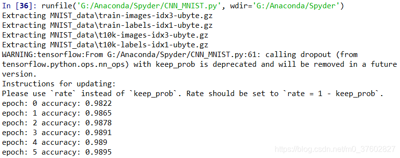
    for epoch in range(6):
        for batch in range(batch_num):
            x_,y_=mnist.train.next_batch(batch_size)
            sess.run(train,feed_dict={x:x_,y:y_,keep_prob:0.7})
        acc=sess.run(accuracy,feed_dict=test_feed)
        print("epoch:",epoch,"accuracy:",acc)

​ 声明：本文转自使用CNN实现MNIST数据集分类