

自然语言建模与词向量
1 统计学语言模型
自然语言处理(Natural Language Processing,NLP)中最基本的问题是:如何计算一个单词(或一段单词序列)在某种语言下出现的概率?即,下文连乘概率式每一项的求取问题。
对于一段拥有T个单词的序列S=(w1,w2,...,wT),计算它出现的概率如下:
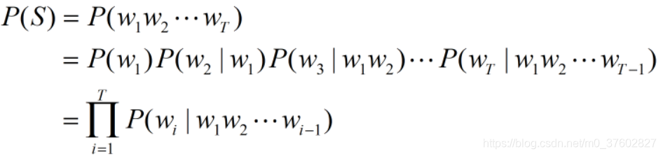
我们知道,每一门语言都有庞大的词汇量,这样的计算方式会造成巨大的参数空间,所以这个原始模型并没有被广泛应用。更多情况下采用这个模型的简化版本——n-gram模型。
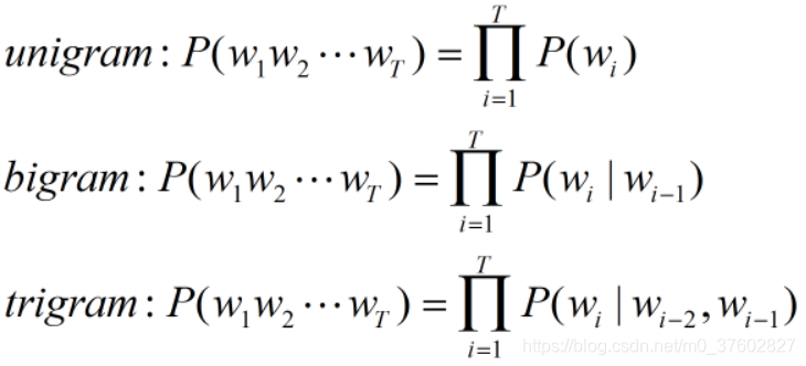
n-gram模型假设当前单词的出现概率仅仅与前面的n-1个单词存在依赖关系。
根据n的取值,可分为unigram(n=1)、bigram(n=2)、trigram(n=3),如下:
2 Word2Vec
Google公司在2013年开放了Word2Vec这一款用于训练词向量的开源软件工具。Word2Vec模型可以根据给定的语料库,通过优化后的训练模型快速有效地将一个词语表达成实数值的向量形式,它可以通过利用词的上下文信息把对文本内容的处理简化为K维向量运算,而向量空间上的相似度可以用来表示文本语义上的相似度。Word2Vec输出的词向量可以用来做很多NLP相关的工作,比如情感分类、找近义词、词性分析等。
Word2Vec有两个实现模式,即CBOW(Continuous Bag Of Word)和Skip-Gram。CBOW是从原始语句中推测目标词,Skip-Gram从目标词推测原始语句。若用w表示目标词,contex(w)表示w的上下文,则CBOW的训练样本为(contex(w),w),Skip-Gram的训练样本为(w,contex(w))。
所谓词向量,即将一个词映射到一个n维空间中的一个点,这样每个词都与一个n维向量对应,任意两个单词间的相似度就可以用向量的余弦相似度来度量。
3 使用Skip-Gram模式实现词向量学习
3.1 语料库
本博客使用的语料库是text8.zip,这是一个不带标点符号的纯文本文件,有17005207个单词,下面展示了部分内容:
anarchism originated as a term of abuse first used against early working class radicals including
the diggers of the english revolution and the sans culottes of the french revolution whilst the term
is still used in a pejorative way to describe any act that used
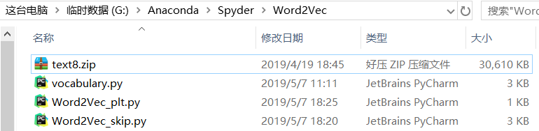
下载text8.zip文件后,无需解压,放在工作目录下,笔者工作目录如下:
3.2 获取训练样本
本博客使用Skip-Gram模型训练词向量,并假设目标单词出现的概率只与它前面的一个单词相关,即采用unigram。
算法步骤如下:
- 创建词汇表并编码词汇表:以语料库中出现频数最高的前49999个单词+单词"unknown"(表示不在词汇表中的单词)定义词汇表(即词汇表中只有50000个单词),按出现频率的高低依次编码为1,2,...,49999,“unknown”编码为0。使用字典count存储词汇表中映射:单词->词频,字典dictionary存储词汇表中映射:单词->编码,字典reverse_dictionary存储词汇表中映射:编码->单词;
- 编码语料库:使用词汇表中的编码规则对语料库进行编码,存储在列表data中;
- 将列表data中的每个编码与它相邻的编码组成有序数对,作为训练样本。以下是语料库中前6个单词生成的8个训练样本:
anarchism originated as a term of abuse first used against early working class radicals

    (3082,12)   ->  (originated,as)
    (3082,5237) ->  (originated,anarchism)
    (12,3082)   ->  (as,originated)
    (12,6)      ->  (as,a)
    (6,195)     ->  (a,term)
    (6,12)      ->  (a,as)
    (195,6)     ->  (term,a)
    (195,2)     ->  (term,of)
vocabulary.py
import tensorflow as tf
import numpy as np
import collections
import random
import zipfile

#返回原始单词列表
def read_data(file):
    with zipfile.ZipFile(file=file) as f:
        original_data = tf.compat.as_str(f.read(f.namelist()[0])).split()
    return original_data

#将原始单词进行编码
def build_vocabulary(original_words):
    count = [["unkown", -1]] #单词-->词频(top50000)
    #统计词频在前50000单词的频数
    count.extend(collections.Counter(original_words).most_common(vocabulary_size-1))
    dictionary = dict() #单词-->词频排名(top50000)
    #将词频在前50000的单词按频数高低依次编号
    for word, _ in count:
        dictionary[word] = len(dictionary)
    data = list() #原始数据的词频排名
    unkown_count = 0
    #建立原始单词到单词编号的映射
    for word in original_words:
        if word in dictionary:
            index = dictionary[word]
        else:
            index = 0
            unkown_count += 1
        data.append(index)
    count[0][1] = unkown_count
    #词频排名-->单词(top50000)
    reverse_dictionary = dict(zip(dictionary.values(), dictionary.keys()))
    return data, count, dictionary, reverse_dictionary

#生成训练批次
def generate_batch(batch_size, num_of_samples, skip_distance):
    global data_index #单词列表索引
    batch = np.ndarray(shape=(batch_size), dtype=np.int32)
    labels = np.ndarray(shape=(batch_size, 1), dtype=np.int32)
    num_of_sample_words = 2 * skip_distance + 1
    #暂存来自data的编号
    buffer = collections.deque(maxlen=num_of_sample_words)
    for _ in range(num_of_sample_words):
        buffer.append(data[data_index])
        data_index = (data_index + 1)
    for i in range(batch_size // num_of_samples):
        target = skip_distance
        #生成样本时需要避免的单词列表
        targets_to_avoid = [skip_distance]
        for j in range(num_of_samples):
            while target in targets_to_avoid:
                target = random.randint(0, num_of_sample_words - 1)
            targets_to_avoid.append(target)
            batch[i * num_of_samples + j] = buffer[skip_distance]
            labels[i * num_of_samples + j, 0] = buffer[target]
        buffer.append(data[data_index]) #当队列满时,再插入元素,会删除队首元素
        data_index = (data_index + 1)
    return batch, labels

#导入语料库
vocabulary_size=50000 #出现频率最高的50000词作为单词表
file="text8.zip" #语料库文件
original_words=read_data(file) #原始单词列表
data_index=0 #单词列表索引
data, count, dictionary, reverse_dictionary=build_vocabulary(original_words)
3.2 训练词向量嵌入矩阵
创建了词汇表后,定义以词汇表中的单词为字典空间(50000维)中的一组基,语料库中的任意一个单词都可以用这组基线性表示。好比人的情感由4个基本情感表示:喜、怒、哀、乐,定义(喜,怒,哀,乐)为情感空间中的一组基,那么其他情感都可以用这组基线性表示,比如:怨 =(0,0.6,0.4,0)。
训练词向量的结果是为了得到一个线性变换T,其矩阵表示为A(50000*128),将词汇表中的50000个单词映射到128维的空间中。设向量x是词汇表中某个单词的编码的one-hot形式(50000维),经映射T后得到词向量y(128维),即y=T(x)=xA。
训练时,损失函数采用的是tf.nn.nce_loss()函数,关于NCE(Noise Constrastive Estimation)模型,详见word2vec 中的数学原理详解(五)基于 Negative Sampling 的模型
Word2Vec_skip.py
import tensorflow as tf
import numpy as np
import math
import vocabulary
max_steps = 100000 #训练最大迭代次数10w次
batch_size = 128
embedding_size = 128 #嵌入向量的尺寸
skip_distance = 1 #相邻单词数
num_of_samples = 2 #对每个单词生成多少样本
vocabulary_size = 50000 #词汇量
num_sampled = 64 #训练时用来做负样本的噪声单词的数量
#16个生成100以内不重复的数字
valid_examples = np.random.choice(100, 16, replace=False)
train_inputs = tf.placeholder(tf.int32, shape=[batch_size])
train_labels = tf.placeholder(tf.int32, shape=[batch_size, 1])
#50000个高频词的嵌入向量
embeddings = tf.Variable(tf.random_uniform([vocabulary_size, embedding_size], -1.0, 1.0))
#获取单词对应的嵌入向量
embed = tf.nn.embedding_lookup(embeddings, train_inputs)
nce_weights = tf.Variable(tf.truncated_normal([vocabulary_size,embedding_size],stddev=1./math.sqrt(embedding_size)))
nce_biases = tf.Variable(tf.zeros([vocabulary_size]))
nec_loss = tf.nn.nce_loss(weights=nce_weights, biases=nce_biases,
inputs=embed, labels=train_labels,
num_sampled=num_sampled,
num_classes=vocabulary_size)
loss = tf.reduce_mean(nec_loss)
train = tf.train.GradientDescentOptimizer(1.0).minimize(loss)
#embeddings行向量L2范数
norm = tf.sqrt(tf.reduce_sum(tf.square(embeddings), 1, keep_dims=True))
#embeddings行向量归一化
normalized_embeddings = embeddings/norm
# 在标准化后的所有单词的词向量值中寻找随机抽取的16个单词对应的词向量值
valid_inputs = tf.constant(valid_examples, dtype=tf.int32)
valid_embeddings = tf.nn.embedding_lookup(normalized_embeddings, valid_inputs)
#计算余弦相似度
similarity = tf.matmul(valid_embeddings, normalized_embeddings, transpose_b=True)
# 开始训练
with tf.Session() as sess:
tf.global_variables_initializer().run()
for step in range(max_steps+1):
batch_inputs,batch_labels=vocabulary.generate_batch(batch_size,num_of_samples,skip_distance)
sess.run(train,feed_dict={train_inputs:batch_inputs,train_labels:batch_labels})
final_embeddings = normalized_embeddings.eval() #标准化嵌入向量
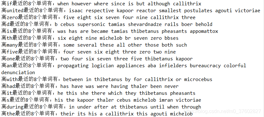
#打印与验证单词最相似的8个单词
similar = similarity.eval()
for i in range(16):
nearest=(-similar[i,:]).argsort()[1:8+1]
valid_word=vocabulary.reverse_dictionary[valid_examples[i]]
nearest_information="离%s最近的8个单词有:"%valid_word
for j in range(8):
close_word=vocabulary.reverse_dictionary[nearest[j]]
nearest_information+=close_word+" "
print(nearest_information)
3.3 绘制词向量空间
由于词向量空间是128维的,并不能直观感知词向量空间,采用TSNE(t-distributed stochastic neighbor embedding)降至2维,再绘制散点图,使其可视化。本博客仅显示了100个词向量。
Word2Vec_plt.py
from sklearn.manifold import TSNE
import matplotlib.pyplot as plt
import vocabulary
import Word2Vec_skip

plot_only=100 #绘制点数

tsne=TSNE(perplexity=30, n_components=2, init="pca", n_iter=5000)
#将128维的嵌入向量降至2维
low_dim_embs=tsne.fit_transform(Word2Vec_skip.final_embeddings[:plot_only,:])

labels=list()
for i in range(plot_only):
    labels.append(vocabulary.reverse_dictionary[i])

plt.figure(figsize=(20,20))
for j,label in enumerate(labels):
    x,y=low_dim_embs[j,:]
    plt.scatter(x,y)
    plt.annotate(label,xy=(x,y),xytext=(2,2),textcoords="offset points") #给嵌入向量点标注注释

#以png格式保存图片
plt.savefig("after_tsne.png")
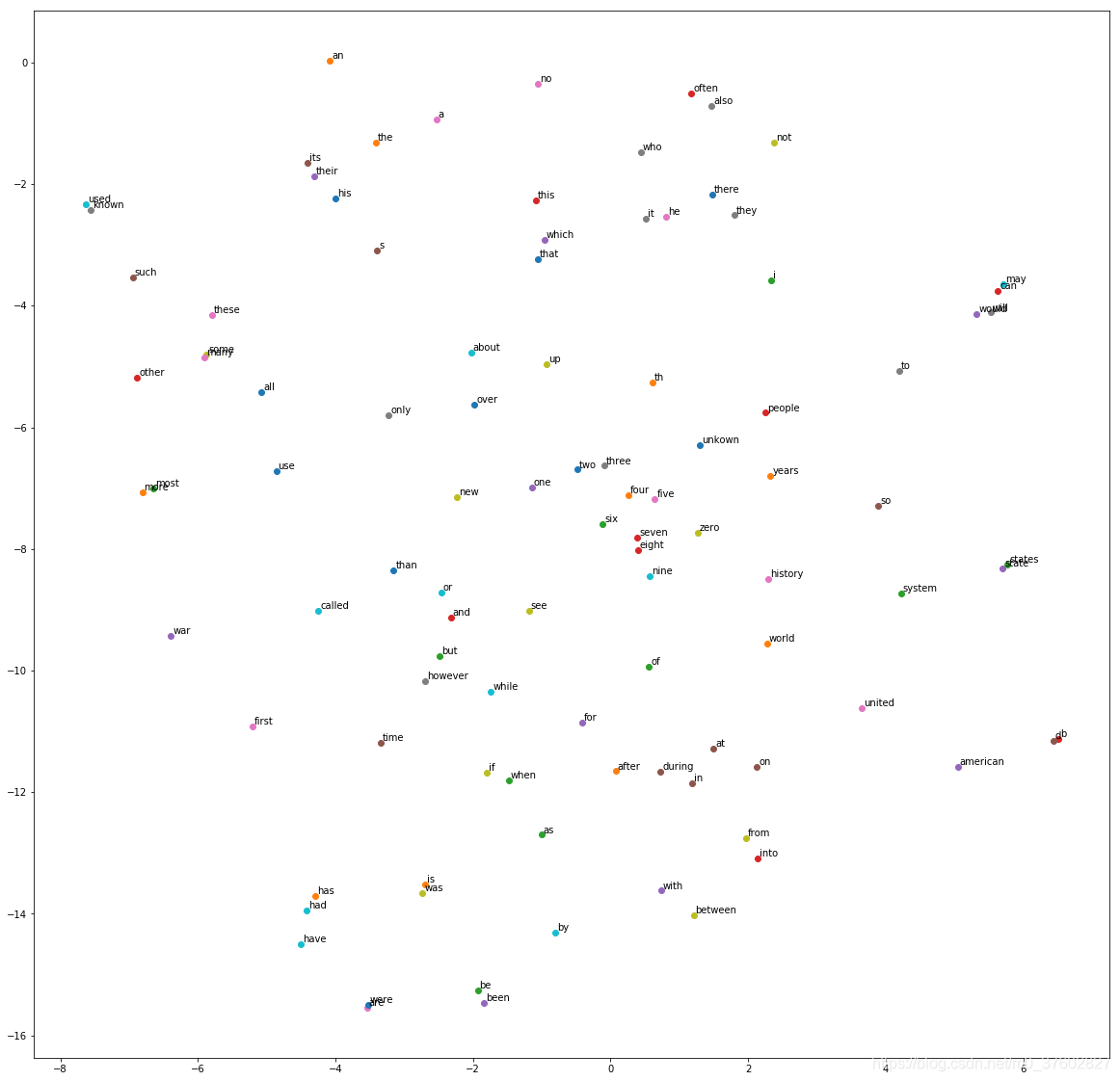
从图中可以看到,词义相近的词在空间上的距离较近,比如右边的“may”、“can”、“would”、“will”,中间的“four”、“five”、“six”、“seven”、“eight”。
声明:本文转自自然语言建模与词向量


【推荐】国内首个AI IDE,深度理解中文开发场景,立即下载体验Trae
【推荐】编程新体验,更懂你的AI,立即体验豆包MarsCode编程助手
【推荐】抖音旗下AI助手豆包,你的智能百科全书,全免费不限次数
【推荐】轻量又高性能的 SSH 工具 IShell:AI 加持,快人一步
· 分享4款.NET开源、免费、实用的商城系统
· 全程不用写代码,我用AI程序员写了一个飞机大战
· MongoDB 8.0这个新功能碉堡了,比商业数据库还牛
· 白话解读 Dapr 1.15:你的「微服务管家」又秀新绝活了
· 上周热点回顾(2.24-3.2)