我眼中的正则化(Regularization)
警告:本文为小白入门学习笔记
在机器学习的过程中我们常常会遇到过拟合和欠拟合的现象,就如西瓜书中一个例子:
如果训练样本是带有锯齿的树叶,过拟合会认为树叶一定要带有锯齿,否则就不是树叶。而欠拟合则认为只要是绿色的就是树叶,会把一棵数也误认为树叶。
过拟合:如果我们的数据集有很多的属性,假设函数会对训练集拟合的非常好,也就是说损失函数J(theta)趋近于零,但是对新的样本却不能较为精确的预测(也就是不能够泛化到一般)。
所以要解决过拟合问题(addressing overfitting):
Options:
1 减少属性的个数
对于那些关联性比较弱的属性可以去掉
2 Regularization(正则化)
过拟合现象的产生可能是我们用这样一个多元方程去拟合实际上是一个一元或二元曲线
![]()
所以我们希望theta3,theta4,theta5竟可能的小,想想如果这样的话曲线是不是会变得简单很多,但是在实际情况下,我们不知道要去减小(penalty)哪一个theta,因此干脆去penalty每一个theta,所以在损失函数后面增加一个项来实现,而这一项就是正则化项

这里我们要记住的是,我们希望损失函数竟可能的小。
而 λ 这个正则化参数需要控制的是这两者之间的平衡,即平衡拟合训练的目标和保持参数值较小的目标。从而来保持假设的形式相对简单,来避免过度的拟合。
首先解决线性回归问题的过拟合:
数据下载:
使用正规方程去求解正规化线性回归是:
![\begin{displaymath}
\theta=(X^{T}X+\lambda\left[\begin{array}{cccc}
0\\
& 1\\
& & \ddots\\
& & & 1\end{array}\right])^{-1}X^{T}\vec{y}\end{displaymath}](http://openclassroom.stanford.edu/MainFolder/courses/DeepLearning/exercises/ex5/img7.png)
跟随 ![]() 后面的是一个(n+1)*(n+1)矩阵,n表示属性的个数
后面的是一个(n+1)*(n+1)矩阵,n表示属性的个数
![\begin{displaymath}
\begin{array}{cc}
\par
\vec{y} = \left[
\begin{array}{c}
y...
...m)})^T\mbox{-}
\end{array}\right] \nonumber
\par
\end{array}\end{displaymath}](http://openclassroom.stanford.edu/MainFolder/courses/DeepLearning/exercises/ex5/img12.png)
使用这个式子就可以计算出theta的值。
MATLAB代码:
function [jVal] = regLinerReg(lamda)
x = load('ex5Linx.dat');
y = load('ex5Liny.dat');
%显示原始数据
plot(x,y,'o','MarkerEdgeColor','b','MarkerFaceColor','r');hold on;
x = [ones(length(y), 1), x, x.^2, x.^3, x.^4, x.^5];
[m,n] = size(x);
n = n - 1;
rm = diag([0;ones(n,1)]);%lamda后面的矩阵
theta = inv(x'*x + lamda .* rm) * x' * y;
disp(theta);
x = load('ex5Linx.dat');
h = theta(1) + theta(2)*x + theta(3)*x.^2 + theta(4)*x.^3 + theta(5)*x.^4 + theta(6)*x.^5;
plot(x(1:m),h,'g-');hold on;
end
分别使正则化参数设置为以下值:
lamda = 0;
lamda = 1;
lamda = 10;
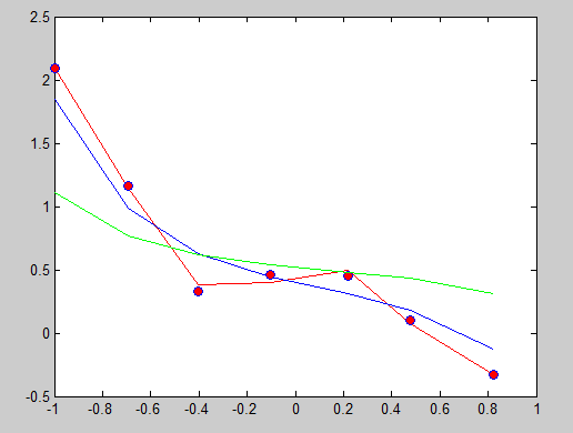
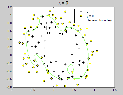
可以发现当lamda=0 时,相当于没有加正则化项,函数经过每一个点,这就是过拟合。lamda = 1时稍微缓和,lamda=10 时函数平和,如果lamda再设置大些,函数曲线可能会成为一条直线。
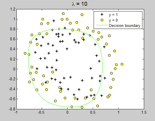
Regularized logistic regression:
拿到数据集后,用MATLAB画出图形:
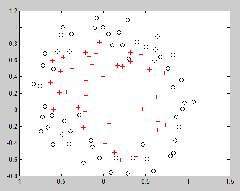
可以看出,这个图并不像前面的可以直接线性分割,所以假设函数是二元,最高次为6次函数。
![\begin{displaymath}
x=\left[\begin{array}{c}
1\\
u\\
v\\
u^2\\
uv\\
v^2\\
u^3\\
\vdots\\
uv^5\\
v^6\end{array}\right]
\end{displaymath}](http://openclassroom.stanford.edu/MainFolder/courses/DeepLearning/exercises/ex5/img29.png)
设u表示x1(也就是数据集ex5Log.dat的第一例数据),v为x2(是第二列数据)。
% Exercise 5 -- Regularized Logistic Regression

clear all; close all; clc

x = load('ex5Logx.dat');
y = load('ex5Logy.dat');


% Plot the training data
% Use different markers for positives and negatives
figure
pos = find(y); neg = find(y == 0);
plot(x(pos, 1), x(pos, 2), 'k+','LineWidth', 2, 'MarkerSize', 7)
hold on
plot(x(neg, 1), x(neg, 2), 'ko', 'MarkerFaceColor', 'y', 'MarkerSize', 7)


% Add polynomial features to x by
% calling the feature mapping function
% provided in separate m-file
x = map_feature(x(:,1), x(:,2)); %获得一个117*28矩阵 117是数据的条数,28是x

[m, n] = size(x);

% Initialize fitting parameters
theta = zeros(n, 1);%28*1

% Define the sigmoid function
g = inline('1.0 ./ (1.0 + exp(-z))');

% setup for Newton's method
MAX_ITR = 15;
J = zeros(MAX_ITR, 1);

% Lambda is the regularization parameter
lambda = 0;

% Newton's Method
for i = 1:MAX_ITR
    % Calculate the hypothesis function
    z = x * theta;
    h = g(z);

    % Calculate J (for testing convergence)
    J(i) =(1/m)*sum(-y.*log(h) - (1-y).*log(1-h))+ ...
    (lambda/(2*m))*norm(theta([2:end]))^2;

    % Calculate gradient and hessian.
    G = (lambda/m).*theta; G(1) = 0; % extra term for gradient
    L = (lambda/m).*eye(n); L(1) = 0;% extra term for Hessian
    grad = ((1/m).*x' * (h-y)) + G;
    H = ((1/m).*x' * diag(h) * diag(1-h) * x) + L;

    % Here is the actual update
    theta = theta - H\grad;

end
% Show J to determine if algorithm has converged
J
% display the norm of our parameters
norm_theta = norm(theta)

% Plot the results
% We will evaluate theta*x over a
% grid of features and plot the contour
% where theta*x equals zero

% Here is the grid range
u = linspace(-1, 1.5, 200);
v = linspace(-1, 1.5, 200);

z = zeros(length(u), length(v));
% Evaluate z = theta*x over the grid
for i = 1:length(u)
    for j = 1:length(v)
        z(i,j) = map_feature(u(i), v(j))*theta;
    end
end
z = z'; % important to transpose z before calling contour

% Plot z = 0
% Notice you need to specify the range [0, 0]
contour(u, v, z, [0, 0], 'LineWidth', 2)
legend('y = 1', 'y = 0', 'Decision boundary')
title(sprintf('\\lambda = %g', lambda), 'FontSize', 14)


hold off

% Uncomment to plot J
% figure
% plot(0:MAX_ITR-1, J, 'o--', 'MarkerFaceColor', 'r', 'MarkerSize', 8)
% xlabel('Iteration'); ylabel('J')
运行结果:
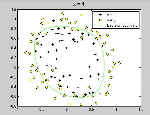
改变lambda = 1
lambda = 10;