第二周作业：多层感知机

多层感知机

线性回归+基础优化方法

1. 模型

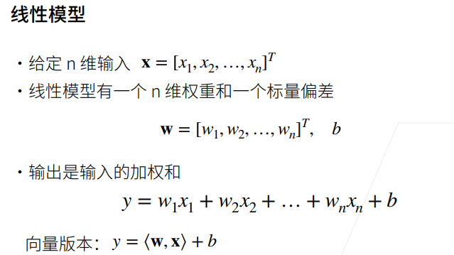
线性回归假设输出与各个输入是线性关系，我们需要建立基于输入\(x_1\)到\(x_n\)来计算输出\(y\)的表达式，也就是模型。

2. 模型训练

通过数据来寻找特定的模型参数值，使模型在数据上的误差尽可能小。这个过程叫模型训练。

3. 损失函数

损失函数能够量化目标的实际值与预测值之间的差距。通常选择非负数作为损失，且数值越小表示损失越小。回归问题中最常用的损失函数是平方误差函数。平方误差可以定义为以下公式：

\[l^{(i)}(w_1,w_2,b)=\frac{1}{2}(\widehat{y}^{(i)}-y^{(i)})^2 \]

通常用训练数据集中所有样本误差的平均来衡量模型预测的质量。模型训练主要是为了找出一组参数使样本平均损失最小。

4. 优化算法

线性回归模型有解析解，但大多数深度学习模型没有解析解，只能通过优化算法有限次迭代模型参数尽可能降低损失函数的值，这类解叫数值解。
梯度下降（gradient descent）法几乎可以优化所有深度学习模型。它通过不断地在损失函数递减的方向上更新参数来降低误差。总结一下，算法的步骤如下：（1）初始化模型参数的值，如随机初始化；（2）从数据集中随机抽取小批量样本且在负梯度的方向上更新参数，并不断迭代这一步骤。

5. 代码实现

5.1 导入包并构造数据集

%matplotlib inline
import random
import torch
from d2l import torch as d2l
#根据带有噪声的线性模型构造一个人造数据集
#线性模型参数w=[2，-3.4]T、b=4.2和噪声项c生成样本数1000的数据集及其标签y=Xw+b+c本次实验为y=w1*x1+w2*x2+b+c
def synthetic_data(w,b,num_examples):
    #生成y=Xw+b+c.
    X=torch.normal(0,1,(num_examples,len(w)))#生成随机矩阵，n个样本，列数为w长度。均值为0，方差为1。
    y=torch.matmul(X,w)+b          #y=Xw+b
    #print(torch.normal(0,0.01,y.shape))
    #print(X,y)
    y+=torch.normal(0,0.01,y.shape)     #均值为0方差为0.01的噪声
    return X,y.reshape((-1,1))       #返回列向量
true_w=torch.tensor([2,-3.4])
true_b=4.3
features,labels=synthetic_data(true_w,true_b,1000)
d2l.set_figsize()
d2l.plt.scatter(features[:,0].detach().numpy(),labels.detach().numpy(),1) #分离出来转为numpy后作图
d2l.plt.scatter(features[:,1].detach().numpy(),labels.detach().numpy(),1) #分离出来转为numpy后作图

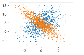
这里蓝色标记点为第一列features与labels作图，橘色为第二列features与labels作图 由于w第一位为正，第二位为负，可以清晰的看出两种点位置的变化趋势。

5.2 读取数据集

'''
data_iter函数，该函数接受批量大小、特征矩阵和标签向量作为输入
生成大小为batch_size的小批量
'''
def data_iter(batch_size,features,labels):
    num_examples=len(features)
    indices=list(range(num_examples)) 
    random.shuffle(indices)#打乱index，使得样本是随机读取的，没有特定的顺序
    for i in range(0,num_examples,batch_size):  #每次i间隔batch_size个数
        batch_indices=torch.tensor(indices[i:min(i+batch_size,num_examples)])
        yield features[batch_indices],labels[batch_indices]  #yield不停返回
batch_size=10  #设置批量大小

5.3 初始化模型参数

w=torch.normal(0,0.01,size=(2,1),requires_grad=True)
b=torch.zeros(1,requires_grad=True)

5.4 定义模型

def linreg(X,w,b):
  #线性回归模型   
  return torch.matmul(X,w)+b

5.5 定义损失函数

def squared_loss(y_hat,y):  #y_hat是预测值 y是真实值
  #损失函数使用均方损失
  return(y_hat-y.reshape(y_hat.shape))**2/2

5.6 定义优化算法

def sgd(params,lr,batch_size):
  #小批量随机梯度下降
  with torch.no_grad():   #禁用梯度计算以加快计算速度
    for param in params:
      param-=lr*param.grad/batch_size
      param.grad.zero_()

5.7训练模型

lr=0.03   #学习率
num_epochs=3   #整个数据扫三遍
net=linreg
loss=squared_loss

for epoch in range(num_epochs):
  for X,y in data_iter(batch_size,features,labels):    #每次拿出批量大小的X和y
    l= loss(net(X,w,b),y)   #放入网络做预测，将预测值与真实值做损失 
                  #l形状为（batch_size,1) 
    l.sum().backward()     #求和求梯度
    sgd([w,b],lr,batch_size)  #使用参数的梯度更新参数
  with torch.no_grad():
    train_l=loss(net(features,w,b),labels)
    print(f'epoch {epoch+1},loss {float(train_l.mean()):f}')

训练结果：

epoch 1,loss 0.029035
epoch 2,loss 0.000112
epoch 3,loss 0.000047

5.8线性回归的简洁实现

#线性回归的简洁实现
import numpy as np
import torch
from torch.utils import data
from d2l import torch as d2l

def synthetic_data(w,b,num_examples): 
  #根据带有噪声的线性模型构造一个人造数据集
  #线性模型参数w=[2，-3.4]T、b=4.2和噪声项c生成数据集及其标签y=Xw+b+c
  X=torch.normal(0,1,(num_examples,len(w)))#生成随机矩阵，n个样本，列数为w长度。均值为0，方差为1。
  y=torch.matmul(X,w)+b          #y=Xw+b
  y+=torch.normal(0,0.01,y.shape)     #均值为0方差为0.01的噪声
  return X,y.reshape((-1,1))       #返回列向量

true_w=torch.tensor([2,-3.4])
true_b=4.2
features,labels=d2l.synthetic_data(true_w,true_b,1000)

def load_array(data_arrays,batch_size,is_train=True):
  #构造一个PyTorch数据迭代器
  #print(type(data_arrays))
  dataset=data.TensorDataset(*data_arrays)   #将数据集传入后生成dataset 
                         #将输入的两类数据进行一一对应
  return data.DataLoader(dataset,batch_size,shuffle=is_train) #随机读取样本
batch_size=10
data_iter=load_array((features,labels),batch_size)
#for i in iter(data_iter):
#  print(type(i))
#iter(data_iter).next()
from torch import nn
net=nn.Sequential(nn.Linear(2,1))  #一个全连接层，输入维度2，输出维度1
net[0].weight.data.normal_(0,0.01)  #通过net[0]访问第一层，通过weight访问w normal为使用正态分布替换data值
net[0].bias.data.fill_(0)  #b为0
loss=nn.MSELoss()  #平方范数求损失
trainer=torch.optim.SGD(net.parameters(),lr=0.03)  #梯度下降

num_epochs=3   #整个数据扫三遍
for epoch in range(num_epochs):
  for X,y in data_iter:
    l=loss(net(X),y)
    trainer.zero_grad()
    l.backward()
    trainer.step()#对模型进行更新
  l=loss(net(features),labels)
  print(f'epoch {epoch+1},loss {l:f}')

训练结果：

epoch 1,loss 0.000221
epoch 2,loss 0.000098
epoch 3,loss 0.000097

Softmax 回归

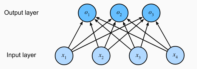
线性回归适用于输出为连续值的情景，当模型输出为离散值时，可以使用softmax等分类模型。但尽管softmax是一个非线性函数，但softmax回归的输出仍然由输入特征的仿射变换决定。因此，softmax回归是一个线性模型。
分类模型：

代码实现

导入包并载入数据集

%matplotlib inline
import torchvision
from torch.utils import data
from torchvision import transforms
import torch
from d2l import torch as d2l
d2l.use_svg_display()
#通过ToTensor实例将图像数据从PIL类型变换成32位浮点数格式
#并除以255使得所有像素的数值均在0到1之间
trans=transforms.ToTensor()
mnist_train=torchvision.datasets.FashionMNIST(root="../data",train=True,transform=trans,download=True)
mnist_test=torchvision.datasets.FashionMNIST(root="../data",train=False,transform=trans,download=True)
print(len(mnist_train),len(mnist_test))
mnist_train[0][0].shape

从输出结果可以看出，图像大小为28*28的单通道图像，训练集为60000张图片，验证集为10000张

查看数据集样例

def get_fashion_mnist_labels(labels):  
    """返回Fashion-MNIST数据集的文本标签。"""
    text_labels = [
        't-shirt', 'trouser', 'pullover', 'dress', 'coat', 'sandal', 'shirt',
        'sneaker', 'bag', 'ankle boot']
    return [text_labels[int(i)] for i in labels]

def show_images(imgs,num_rows,num_cols,titles=None,scale=1.5):
  '''Plot a list of images.'''
  figsize=(num_cols*scale,num_rows*scale)
  _, axes = d2l.plt.subplots(num_rows, num_cols, figsize=figsize)
  axes = axes.flatten()
  for i, (ax, img) in enumerate(zip(axes, imgs)):
    if torch.is_tensor(img):
      ax.imshow(img.numpy())
    else:
      ax.imshow(img)
    ax.axes.get_xaxis().set_visible(False)
    ax.axes.get_yaxis().set_visible(False)
    if titles:
      ax.set_title(titles[i])
  return axes
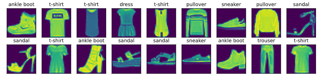
#几个样本的图像及其相应的标签
X, y = next(iter(data.DataLoader(mnist_train, batch_size=18)))
show_images(X.reshape(18, 28, 28), 2, 9, titles=get_fashion_mnist_labels(y));

测试读数据时间并初始化模型参数

batch_size=256
def get_dataloader_workers():
  #使用四个进程读取数据
  return 4
train_iter=data.DataLoader(mnist_train,batch_size,shuffle=True,num_workers=get_dataloader_workers())
timer=d2l.Timer()
for X,y in train_iter:
  continue
f'{timer.stop():.2f} sec'
import torch
from IPython import display
from d2l import torch as d2l
batch_size=256
num_inputs=784
num_outputs=10
train_iter,test_iter=d2l.load_data_fashion_mnist(batch_size)
W=torch.normal(0,0.01,size=(num_inputs,num_outputs),requires_grad=True)
b=torch.zeros(num_outputs,requires_grad=True)

定义softmax模型

def softmax(X):
  X_exp=torch.exp(X)
  partition=X_exp.sum(1,keepdim=True)
  return X_exp/partition
def net(X):
  #softmax回归模型
  return softmax(torch.matmul(X.reshape(-1,W.shape[0]),W)+b)

定义交叉熵损失函数及预测准确率函数

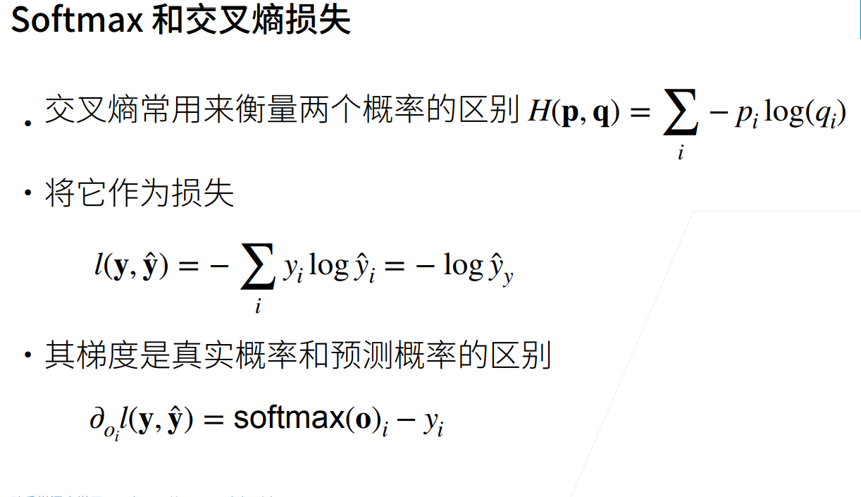
def cross_entropy(y_hat,y):
  #交叉熵损失函数，可以使用平方损失，但是只需要分类结果预测正确
  #平方损失过于严格，使用交叉熵损失
  return -torch.log(y_hat[range(len(y_hat)),y])
def accuracy(y_hat,y):
  '''计算预测正确的数量'''
  if len(y_hat.shape)>1 and y_hat.shape[1]>1:
    y_hat=y_hat.argmax(axis=1)
    #print(y_hat)
  cmp=y_hat.type(y.dtype)==y
  #print(cmp)
  #cmp=cmp.type(y.dtype)
  #print(cmp)
  return float(cmp.type(y.dtype).sum())
def evaluate_accuracy(net,data_iter):
  '''计算在指定数据集上模型的精度'''
  if isinstance(net,torch.nn.Module):
    net.eval() #将模型设置为评估模式
  metric=Accumulator(2)  #正确预测数，预测总数
  for X,y in data_iter:
    #print(metric[1])
    metric.add(accuracy(net(X),y),y.numel())
  #print(y.numel())
  #print(metric[1])
  return metric[0]/metric[1]
class Accumulator:  
    """在`n`个变量上累加。"""
    def __init__(self, n):
        self.data = [0.0] * n

    def add(self, *args):
        self.data = [a + float(b) for a, b in zip(self.data, args)]

    def reset(self):
        self.data = [0.0] * len(self.data)

    def __getitem__(self, idx):
        return self.data[idx]

evaluate_accuracy(net, test_iter)

定义训练模型

def train_epoch_ch3(net,train_iter,loss,updater):
  if isinstance(net,torch.nn.Module):
    net.train()
  metric=Accumulator(3)
  for X,y in train_iter:
    y_hat=net(X)
    l=loss(y_hat,y)
    if isinstance(updater,torch.optim.Optimizer):#isinstance() 函数来判断一个对象是否是一个已知的类型，类似 type()。
      updater.zero_grad()
      l.backward()
      updater.step()
      print(len(y))
      metric.add(float(1)*len(y),accuracy(y_hat,y),y.size().numel())
    else:
      l.sum().backward()
      updater(X.shape[0])
      metric.add(float(l.sum()),accuracy(y_hat,y),y.numel())
  return metric[0]/metric[2],metric[1]/metric[2]

可视化模块

class Animator:  
    """在动画中绘制数据。"""
    def __init__(self, xlabel=None, ylabel=None, legend=None, xlim=None,
                 ylim=None, xscale='linear', yscale='linear',
                 fmts=('-', 'm--', 'g-.', 'r:'), nrows=1, ncols=1,
                 figsize=(3.5, 2.5)):
        if legend is None:
            legend = []
        d2l.use_svg_display()
        self.fig, self.axes = d2l.plt.subplots(nrows, ncols, figsize=figsize)
        if nrows * ncols == 1:
            self.axes = [self.axes,]
        self.config_axes = lambda: d2l.set_axes(self.axes[
            0], xlabel, ylabel, xlim, ylim, xscale, yscale, legend)
        self.X, self.Y, self.fmts = None, None, fmts

    def add(self, x, y):
        if not hasattr(y, "__len__"):
            y = [y]
        n = len(y)
        if not hasattr(x, "__len__"):
            x = [x] * n
        if not self.X:
            self.X = [[] for _ in range(n)]
        if not self.Y:
            self.Y = [[] for _ in range(n)]
        for i, (a, b) in enumerate(zip(x, y)):
            if a is not None and b is not None:
                self.X[i].append(a)
                self.Y[i].append(b)
        self.axes[0].cla()
        for x, y, fmt in zip(self.X, self.Y, self.fmts):
            self.axes[0].plot(x, y, fmt)
        self.config_axes()
        display.display(self.fig)
        display.clear_output(wait=True)

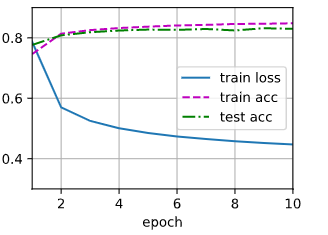
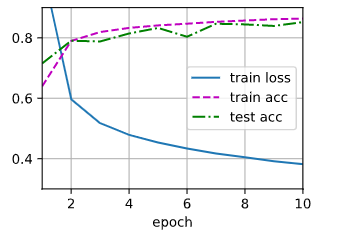
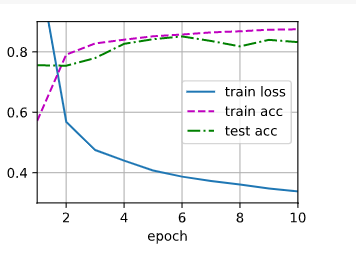
训练模型

def train_ch3(net, train_iter, test_iter, loss, num_epochs, updater):  
    """训练模型。"""
    animator = Animator(xlabel='epoch', xlim=[1, num_epochs], ylim=[0.3, 0.9],
                        legend=['train loss', 'train acc', 'test acc'])
    for epoch in range(num_epochs):
        train_metrics = train_epoch_ch3(net, train_iter, loss, updater)
        test_acc = evaluate_accuracy(net, test_iter)
        animator.add(epoch + 1, train_metrics + (test_acc,))
        #print(train_metrics[0],train_metrics[1])
    train_loss, train_acc = train_metrics

设置优化函数及学习率并训练

lr = 0.1
def updater(batch_size):
    return d2l.sgd([W, b], lr, batch_size)
num_epochs = 10
train_ch3(net, train_iter, test_iter, cross_entropy, num_epochs, updater)

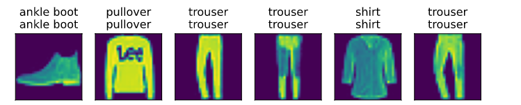
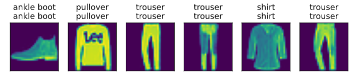
预测结果

def predict_ch3(net, test_iter, n=6):  
    """预测标签（定义见第3章）。"""
    for X, y in test_iter:
        break
    trues = d2l.get_fashion_mnist_labels(y)
    preds = d2l.get_fashion_mnist_labels(net(X).argmax(axis=1))
    titles = [true + '\n' + pred for true, pred in zip(trues, preds)]
    d2l.show_images(X[0:n].reshape((n, 28, 28)), 1, n, titles=titles[0:n])
predict_ch3(net, test_iter)

Softmax简洁实现

#softmax回归的简洁实现
import torch
from torch import nn
from d2l import torch as d2l
batch_size=256
train_iter,test_iter=d2l.load_data_fashion_mnist(batch_size)
#先展平。在全连接层前调整网络输入的形状
net=nn.Sequential(nn.Flatten(),nn.Linear(784,10))
def init_weights(m):
  #初始化参数
  if type(m) == nn.Linear:
    nn.init.normal_(m.weight,std=0.01)
net.apply(init_weights)
#在交叉熵损失函数中传递未归一化的预测，并同时计算softmax及其对数
loss=nn.CrossEntropyLoss()
#使用学习率为0.1的小批量随机梯度下降作为优化算法
trainer=torch.optim.SGD(net.parameters(),lr=0.1)
num_epochs=10
d2l.train_ch3(net,train_iter,test_iter,loss,num_epochs,trainer)

多层感知机

1. 感知机

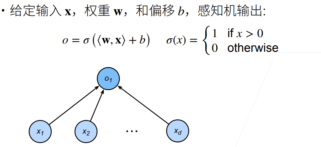
感知机是一个二分类模型。它的求解算法等价于使用批量大小为1的梯度下降，它不能拟合XOR函数，导致了第一次AI寒冬。

2.多层感知机

多层感知机使用隐藏层和激活函数来得到非线性模型。

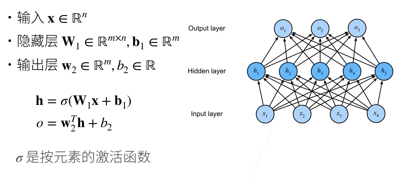
必须使用非线性激活函数，否则输出仍然是输入的线性变换。

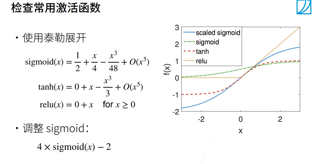
2.1 激活函数

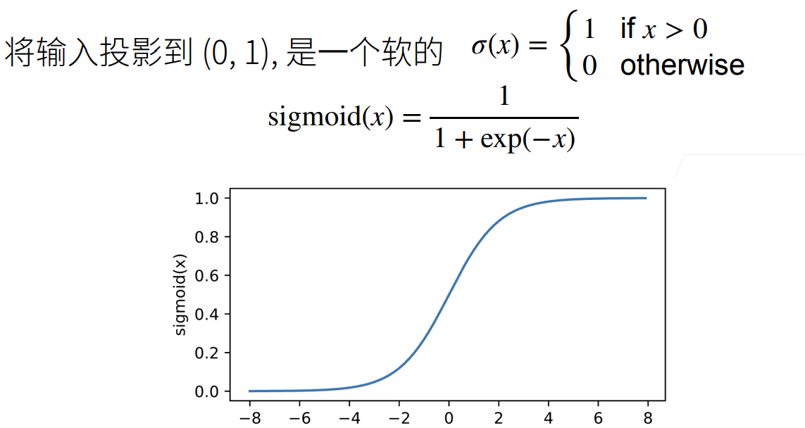
2.1.1 Sigmoid激活函数

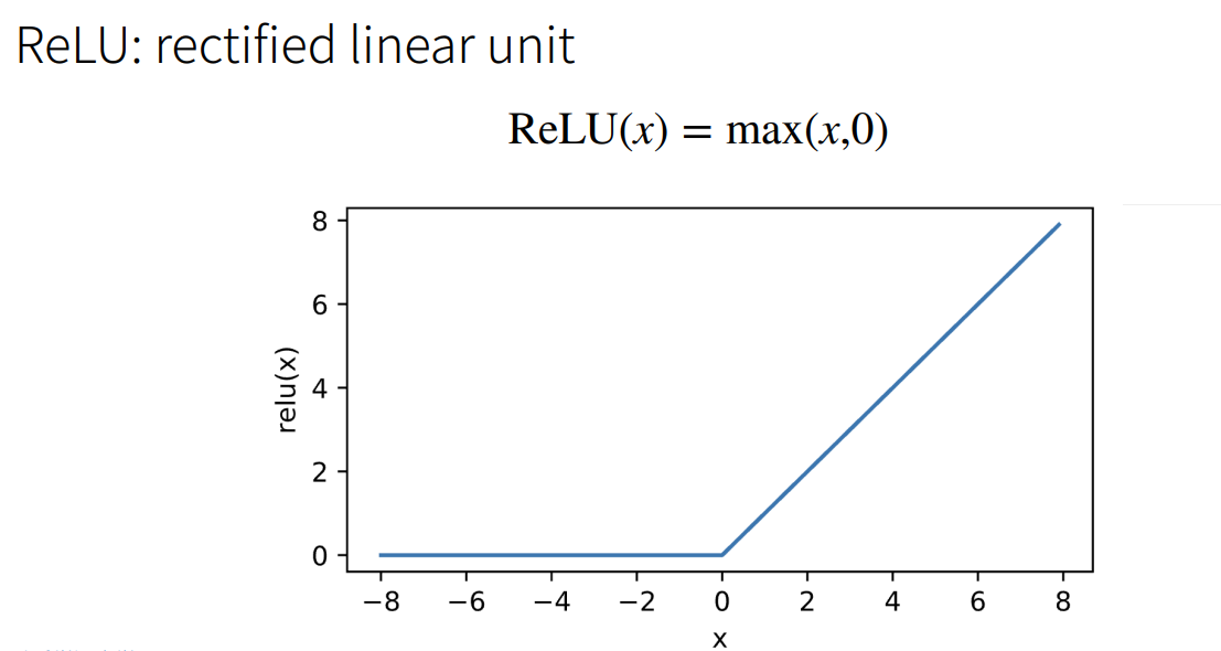
2.1.2 ReLU激活函数

2.1.3 Tanh激活函数

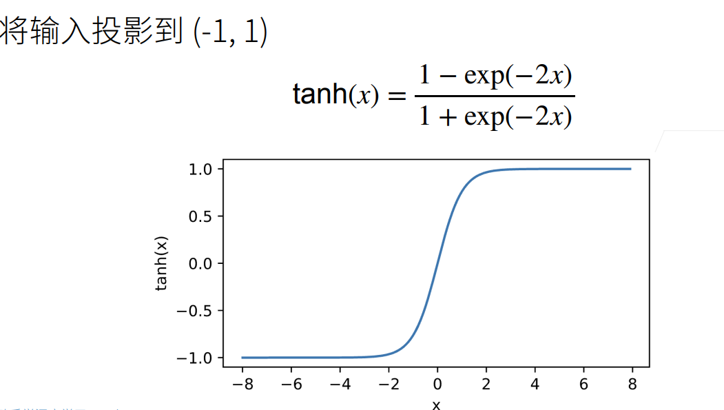
2.2 多层感知机的从零开始实现

2.2.1 初始化模型参数

import torch
from torch import nn
from d2l import torch as d2l
batch_size=256
train_iter,test_iter=d2l.load_data_fashion_mnist(batch_size)
num_inputs,num_outputs,num_hiddens=784,10,256
W1=nn.Parameter(torch.randn(num_inputs,num_hiddens,requires_grad=True) * 0.01)
b1=nn.Parameter(torch.zeros(num_hiddens,requires_grad=True))
W2=nn.Parameter(torch.randn(num_hiddens,num_outputs,requires_grad=True) * 0.01)
b2=nn.Parameter(torch.zeros(num_outputs,requires_grad=True))
params = [W1, b1, W2, b2]

2.2.2 激活函数

def relu(X):
#Relu激活函数
  a=torch.zeros_like(X)
  return torch.max(X,a)

2.2.3 模型

def net(X):
  X=X.reshape((-1,num_inputs))
  H=relu(X@W1+b1)
  return (H@W2+b2)

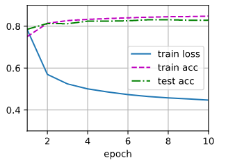
2.2.4 训练并预测

loss=nn.CrossEntropyLoss()
num_epochs,lr=10,0.1
updater=torch.optim.SGD(params,lr=lr)
d2l.train_ch3(net,train_iter,test_iter,loss,num_epochs,updater)
d2l.predict_ch3(net, test_iter)

多层感知机简洁实现

#简洁实现
num_epochs = 10
batch_size=256
#两个全连接层，第一层做非线性处理。
net=nn.Sequential(nn.Flatten(),nn.Linear(784,256),nn.ReLU(),nn.Linear(256,10))
def init_weights(m):
  if type(m) == nn.Linear:
    nn.init.normal_(m.weight,std=0.01)
net.apply(init_weights)
loss = nn.CrossEntropyLoss()
trainer = torch.optim.SGD(net.parameters(), lr=0.1)
train_iter,test_iter=d2l.load_data_fashion_mnist(batch_size)
d2l.train_ch3(net,train_iter,test_iter,loss,num_epochs,trainer)

模型选择，过拟合和欠拟合

1. 训练误差和泛化误差

训练误差（training error）是指，我们的模型在训练数据集上计算得到的误差。
泛化误差（generalization error）是指，当我们将模型应用在同样从原始样本的分布中抽取的无限多的数据样本时，我们模型误差的期望。

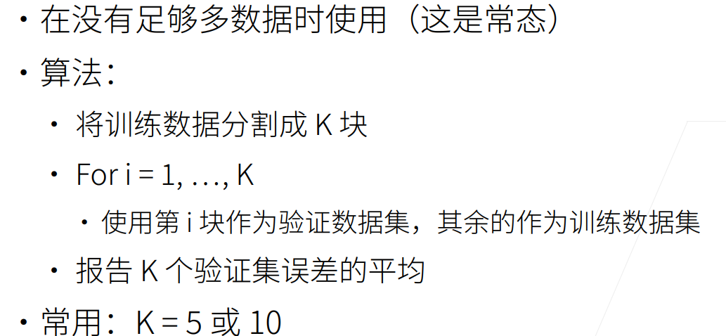
2.K-折交叉验证

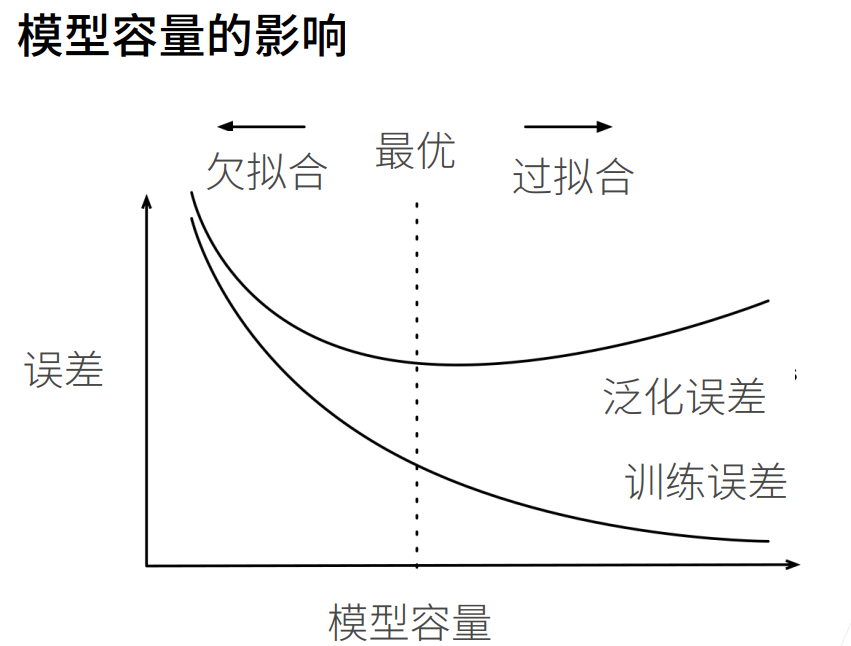
3.欠拟合和过拟合

先用一张表来解释欠拟合与过拟合出现的原因

3.1 模型容量

模型容量指模型拟合各种函数的能力

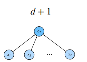
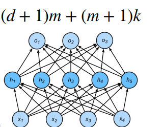
估计模型容量大小的方式有两种：一是参数个数，二是参数值的取值范围。
计算方法:

3.2 总结

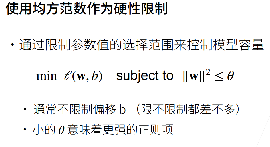
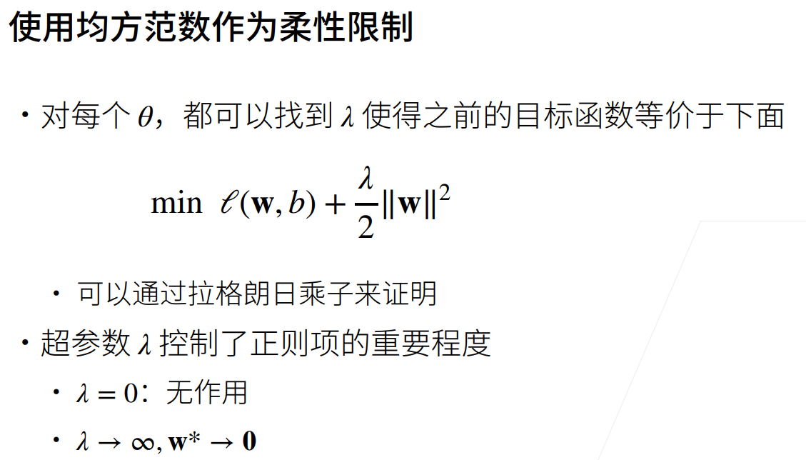
权重衰退与丢弃法

权重衰退

代码实现

读取数据集

%matplotlib inline
import torch
from torch import nn
from d2l import torch as d2l
n_train,n_test,num_inputs,batch_size=20,100,200,5
true_w,true_b=torch.ones((num_inputs,1))*0.01,0.05
train_data=d2l.synthetic_data(true_w,true_b,n_train)
train_iter=d2l.load_array(train_data,batch_size)
test_data=d2l.synthetic_data(true_w,true_b,n_test)
test_iter=d2l.load_array(test_data,batch_size,is_train=False)

定义初始化参数函数

def init_params():
  w=torch.normal(0,1,size=(num_inputs,1),requires_grad=True)
  b=torch.zeros(1,requires_grad=True)
  return [w,b]

定义L2范数惩罚

def l2_penalty(w):
  #定义L2范数惩罚
  return torch.sum(w.pow(2))/2

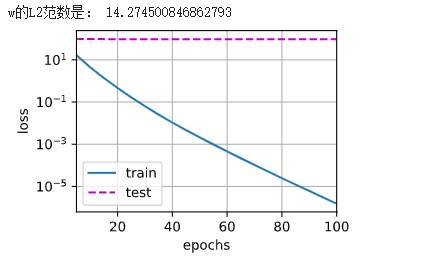
定义训练函数

def train(lambd):
    w, b = init_params()
    net, loss = lambda X: d2l.linreg(X, w, b), d2l.squared_loss
    num_epochs, lr = 100, 0.003
    animator = d2l.Animator(xlabel='epochs', ylabel='loss', yscale='log',
                            xlim=[5, num_epochs], legend=['train', 'test'])
    for epoch in range(num_epochs):
        for X, y in train_iter:
          l = loss(net(X), y) + lambd * l2_penalty(w)
          l.sum().backward()
          d2l.sgd([w, b], lr, batch_size)
        if (epoch + 1) % 5 == 0:
          animator.add(epoch + 1, (d2l.evaluate_loss(net, train_iter, loss),
                        d2l.evaluate_loss(net, test_iter, loss)))
    print('w的L2范数是：', torch.norm(w).item())

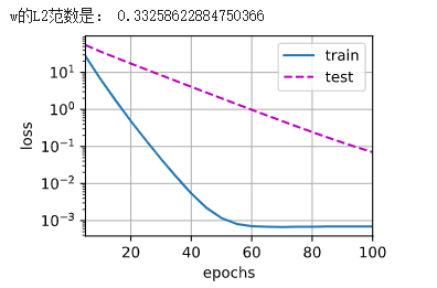
不同权重衰退参数的训练结果

#直接计算
train(lambd=0)

#使用权重衰减
train(lambd=3)

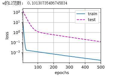
权重衰退简洁实现

只需要在优化函数中设置weight_decay参数即可

def train_concise(wd):
    net = nn.Sequential(nn.Linear(num_inputs, 1))
    for param in net.parameters():
        param.data.normal_()
    loss = nn.MSELoss()
    num_epochs, lr = 500, 0.003
    trainer = torch.optim.SGD([{
        "params": net[0].weight,
        'weight_decay': wd}, {
            "params": net[0].bias}], lr=lr)
    animator = d2l.Animator(xlabel='epochs', ylabel='loss', yscale='log',
                            xlim=[5, num_epochs], legend=['train', 'test'])
    for epoch in range(num_epochs):
        for X, y in train_iter:
            with torch.enable_grad():
                trainer.zero_grad()
                l = loss(net(X), y)
            l.backward()
            trainer.step()
        if (epoch + 1) % 5 == 0:
            animator.add(epoch + 1, (d2l.evaluate_loss(net, train_iter, loss),
                                     d2l.evaluate_loss(net, test_iter, loss)))
    print('w的L2范数：', net[0].weight.norm().item())
train_concise(3)

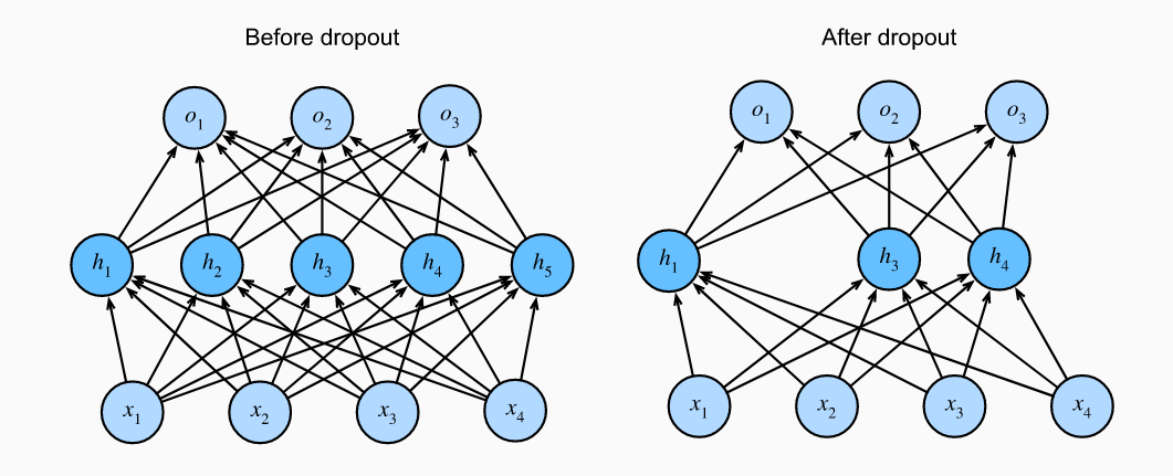
Dropout

Dropout主要用于防止过拟合。常用trick，将模型复杂度加大，再通过正则化控制模型复杂度。可以加深网络，将dropout率设大一些可能比浅层网络效果好。

Dropout原理

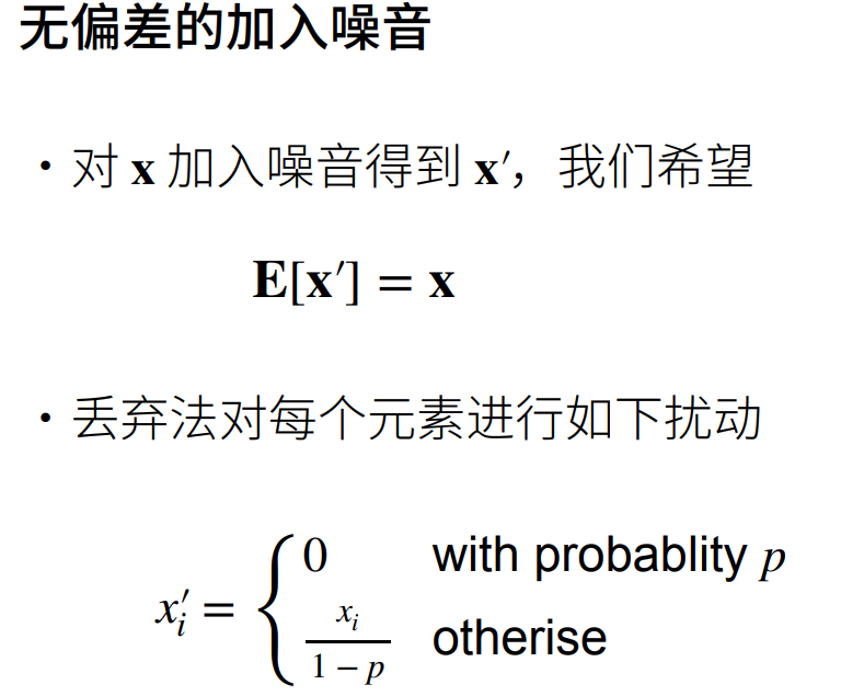
这样做可以保证期望值不变。
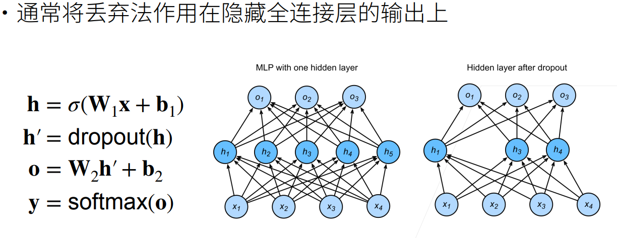
实践中的Dropout

Dropout使用

定义Dropout函数并验证

#dropout
def dropout_layer(X,dropout):
  assert 0<=dropout<=1
  if dropout == 1:
    return torch.zeros_like(X)
  if dropout == 0:
    return X
  mask=(torch.randn(X.shape)>dropout).float()
  return mask*X/(1.0-dropout)
X=torch.arange(16,dtype=torch.float32).reshape((2,8))
print(X)
print(dropout_layer(X,0.))
print(dropout_layer(X,0.5))
print(dropout_layer(X,1.))

tensor([[ 0.,  1.,  2.,  3.,  4.,  5.,  6.,  7.],
        [ 8.,  9., 10., 11., 12., 13., 14., 15.]])
tensor([[ 0.,  1.,  2.,  3.,  4.,  5.,  6.,  7.],
        [ 8.,  9., 10., 11., 12., 13., 14., 15.]])
tensor([[ 0.,  2.,  0.,  0.,  8.,  0., 12., 14.],
        [ 0.,  0.,  0.,  0.,  0.,  0.,  0.,  0.]])
tensor([[0., 0., 0., 0., 0., 0., 0., 0.],
        [0., 0., 0., 0., 0., 0., 0., 0.]])

可以看到，不同参数所进行的不同操作。当p=0.5时，每个元素有一半的几率被丢弃。

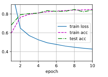
加入Dropout进行训练

#定义具有两个隐藏层的多层感知机，每个隐藏层包含256个单元
num_inputs,num_outputs,num_hiddens1,num_hiddens2=784,10,256,256
dropout1,dropout2=0.2,0.5
class Net(nn.Module):
    def __init__(self, num_inputs, num_outputs, num_hiddens1, num_hiddens2,
                 is_training=True):
        super(Net, self).__init__()
        self.num_inputs = num_inputs
        self.training = is_training
        self.lin1 = nn.Linear(num_inputs, num_hiddens1)
        self.lin2 = nn.Linear(num_hiddens1, num_hiddens2)
        self.lin3 = nn.Linear(num_hiddens2, num_outputs)
        self.relu = nn.ReLU()

    def forward(self, X):
        H1 = self.relu(self.lin1(X.reshape((-1, self.num_inputs))))
        if self.training == True:
            H1 = dropout_layer(H1, dropout1)
        H2 = self.relu(self.lin2(H1))
        if self.training == True:
            H2 = dropout_layer(H2, dropout2)
        out = self.lin3(H2)
        return out

net = Net(num_inputs, num_outputs, num_hiddens1, num_hiddens2) 
num_epochs,lr,batch_size=10,0.5,256
loss=nn.CrossEntropyLoss()
train_iter,test_iter=d2l.load_data_fashion_mnist(batch_size)
trainer=torch.optim.SGD(net.parameters(),lr=lr)
d2l.train_ch3(net,train_iter,test_iter,loss,num_epochs,trainer)

Dropout简洁实现

直接在网络中加入Dropout函数即可。参数为丢弃率

#简洁实现
net=nn.Sequential(nn.Flatten(),nn.Linear(784,256),nn.ReLU(),nn.Dropout(dropout1),
        nn.Linear(256,256),nn.ReLU(),nn.Dropout(dropout2),nn.Linear(256,10))
def init_weights(m):
  if type(m)==nn.Linear:
    nn.init.normal_(m.weight,std=0.01)
net.apply(init_weights)
trainer=torch.optim.SGD(net.parameters(),lr=lr)
d2l.train_ch3(net,train_iter,test_iter,loss,num_epochs,trainer)

数值稳定性和模型初始化

初始化方案的选择在神经网络学习中起着非常重要的作用，它对保持数值稳定性至关重要。

1. 梯度消失和梯度爆炸

梯度消失和梯度爆炸的根源主要是因为深度神经网络结构以及反向传播算法，目前优化神经网络的方法都是基于反向传播的思想，即根据损失函数计算的误差通过反向传播的方式，指导深度网络权值的更新。
由于深度网络是多层非线性函数的堆砌，整个深度网络可以视为是一个复合的非线性多元函数（这些非线性多元函数其实就是每层的激活函数），那么对loss function求不同层的权值偏导，相当于应用梯度下降的链式法则，链式法则是一个连乘的形式，所以当层数越深的时候，梯度将以指数传播。
如果接近输出层的激活函数求导后梯度值大于1，那么层数增多的时候，最终求出的梯度很容易指数级增长，就会产生梯度爆炸；相反，如果小于1，那么经过链式法则的连乘形式，也会很容易衰减至0，就会产生梯度消失。

1.1 梯度消失

梯度消失经常出现。产生的原因有：一是在深层网络中，二是采用了不合适的损失函数，比如sigmoid。当梯度消失发生时，接近于输出层的隐藏层由于其梯度相对正常，所以权值更新时也就相对正常，但是当越靠近输入层时，由于梯度消失现象，会导致靠近输入层的隐藏层权值更新缓慢或者更新停滞。这就导致在训练时，只等价于后面几层的浅层网络的学习。

1.2 梯度爆炸

梯度爆炸一般出现在深层网络和权值初始化值太大的情况下。在深层神经网络或循环神经网络中，误差的梯度可在更新中累积相乘。如果网络层之间的梯度值大于 1.0，那么重复相乘会导致梯度呈指数级增长，梯度变的非常大，然后导致网络权重的大幅更新，并因此使网络变得不稳定。

1.3 打破对称性

神经网络设计中的另一个问题是其参数化所固有的对称性。dropout正则化可以打破这种对称性。

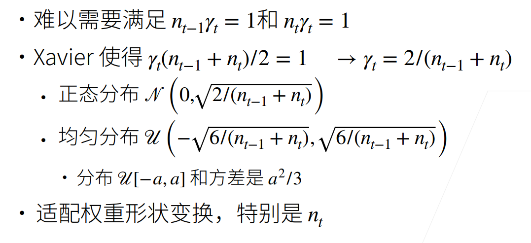
参数初始化

默认初始化

使用正态分布来初始化权重值。

Xavier初始化

实战Kaggle房价预测样例

import hashlib
import os
import tarfile
import zipfile
import requests

DATA_HUB = dict()
DATA_URL = 'http://d2l-data.s3-accelerate.amazonaws.com/'

def download(name, cache_dir=os.path.join('..', 'data')):  
    """下载一个DATA_HUB中的文件，返回本地文件名。"""
    assert name in DATA_HUB, f"{name} 不存在于 {DATA_HUB}."
    url, sha1_hash = DATA_HUB[name]
    os.makedirs(cache_dir, exist_ok=True)
    fname = os.path.join(cache_dir, url.split('/')[-1])
    if os.path.exists(fname):
        sha1 = hashlib.sha1()
        with open(fname, 'rb') as f:
            while True:
                data = f.read(1048576)
                if not data:
                    break
                sha1.update(data)
        if sha1.hexdigest() == sha1_hash:
            return fname
    print(f'正在从{url}下载{fname}...')
    r = requests.get(url, stream=True, verify=True)
    with open(fname, 'wb') as f:
        f.write(r.content)
    return fname

def download_extract(name, folder=None):  
    """下载并解压zip/tar文件。"""
    fname = download(name)
    base_dir = os.path.dirname(fname)
    data_dir, ext = os.path.splitext(fname)
    if ext == '.zip':
        fp = zipfile.ZipFile(fname, 'r')
    elif ext in ('.tar', '.gz'):
        fp = tarfile.open(fname, 'r')
    else:
        assert False, '只有zip/tar文件可以被解压缩。'
    fp.extractall(base_dir)
    return os.path.join(base_dir, folder) if folder else data_dir

def download_all():  
    """下载DATA_HUB中的所有文件。"""
    for name in DATA_HUB:
        download(name)
#使用pandas读入并处理数据
%matplotlib inline
import numpy as np
import pandas as pd
import torch
from torch import nn
from d2l import torch as d2l

DATA_HUB['kaggle_house_train'] = (  
    DATA_URL + 'kaggle_house_pred_train.csv',
    '585e9cc93e70b39160e7921475f9bcd7d31219ce')

DATA_HUB['kaggle_house_test'] = (  
    DATA_URL + 'kaggle_house_pred_test.csv',
    'fa19780a7b011d9b009e8bff8e99922a8ee2eb90')

train_data = pd.read_csv(download('kaggle_house_train'))
test_data = pd.read_csv(download('kaggle_house_test'))

print(train_data.shape)
print(test_data.shape)
#前四行的前四个和最后两个特征，以及相应标签
print(train_data.iloc[0:4, [0, 1, 2, 3, -3, -2, -1]])
print(test_data.iloc[0:4, [0, 1, 2, 3, -3, -2, -1]])
#在每个样本中，第一个特征是ID，将其从数据集中删除
all_features = pd.concat((train_data.iloc[:, 1:-1], test_data.iloc[:, 1:]))
print(all_features)
#清洗数据。将所有缺失的值替换为相应特征的平均值。 通过将特征重新缩放到零均值和单位方差来标准化数据
numeric_features = all_features.dtypes[all_features.dtypes != 'object'].index
all_features[numeric_features] = all_features[numeric_features].apply(
    lambda x: (x - x.mean()) / (x.std()))
all_features[numeric_features] = all_features[numeric_features].fillna(0)
#用独热码编码离散值
all_features = pd.get_dummies(all_features, dummy_na=True)
#从pandas格式中提取NumPy格式，并将其转换为张量表示
n_train = train_data.shape[0]
#print(all_features[:n_train])
train_features = torch.tensor(all_features[:n_train].values,dtype=torch.float32)
test_features = torch.tensor(all_features[n_train:].values,dtype=torch.float32)
train_labels = torch.tensor(train_data.SalePrice.values.reshape(-1, 1),dtype=torch.float32)
loss=MSELoss()
in_feature=train_data.shape[1]
def get_net():
  net=nn.Sequential(nn.Linear(in_feature,1))
  return net
#使用相对误差来衡量差异，有除法取log
def log_rmse(net,features,labels):
  clipped_preds=torch.clamp(net(features),1float('inf'))
  rmse=torch.sqrt(loss(torch.log(clipped_preds),torch.log(labels)))
  return rmse.item()
def train(net, train_features, train_labels, test_features, test_labels,
          num_epochs, learning_rate, weight_decay, batch_size):
    train_ls, test_ls = [], []
    train_iter = d2l.load_array((train_features, train_labels), batch_size)
    optimizer = torch.optim.Adam(net.parameters(), lr=learning_rate,weight_decay=weight_decay)#使用Adamy优化器
    for epoch in range(num_epochs):
        for X, y in train_iter:
            optimizer.zero_grad()
            l = loss(net(X), y)
            l.backward()
            optimizer.step()
        train_ls.append(log_rmse(net, train_features, train_labels))
        if test_labels is not None:
            test_ls.append(log_rmse(net, test_features, test_labels))
    return train_ls, test_ls
#K折交叉验证
def get_k_fold_data(k, i, X, y):
    assert k > 1
    fold_size = X.shape[0] // k
    X_train, y_train = None, None
    for j in range(k):
        idx = slice(j * fold_size, (j + 1) * fold_size)
        X_part, y_part = X[idx, :], y[idx]
        if j == i:
            X_valid, y_valid = X_part, y_part
        elif X_train is None:
            X_train, y_train = X_part, y_part
        else:
            X_train = torch.cat([X_train, X_part], 0)
            y_train = torch.cat([y_train, y_part], 0)
    return X_train, y_train, X_valid, y_valid

#返回训练和验证误差的平均值
def k_fold(k, X_train, y_train, num_epochs, learning_rate, weight_decay,
           batch_size):
    train_l_sum, valid_l_sum = 0, 0
    for i in range(k):
        data = get_k_fold_data(k, i, X_train, y_train)
        net = get_net()
        train_ls, valid_ls = train(net, *data, num_epochs, learning_rate,
                                   weight_decay, batch_size)
        train_l_sum += train_ls[-1]
        valid_l_sum += valid_ls[-1]
        if i == 0:
            d2l.plot(list(range(1, num_epochs + 1)), [train_ls, valid_ls],
                     xlabel='epoch', ylabel='rmse', xlim=[1, num_epochs],
                     legend=['train', 'valid'], yscale='log')
        print(f'fold {i + 1}, train log rmse {float(train_ls[-1]):f}, '
              f'valid log rmse {float(valid_ls[-1]):f}')
    return train_l_sum / k, valid_l_sum / k
#模型选择

k, num_epochs, lr, weight_decay, batch_size = 5, 100, 5, 0, 64
train_l, valid_l = k_fold(k, train_features, train_labels, num_epochs, lr,
                          weight_decay, batch_size)
print(f'{k}-折验证: 平均训练log rmse: {float(train_l):f}, '
      f'平均验证log rmse: {float(valid_l):f}')
#提交Kaggle预测

def train_and_pred(train_features, test_feature, train_labels, test_data,
                   num_epochs, lr, weight_decay, batch_size):
    net = get_net()
    train_ls, _ = train(net, train_features, train_labels, None, None,
                        num_epochs, lr, weight_decay, batch_size)
    d2l.plot(np.arange(1, num_epochs + 1), [train_ls], xlabel='epoch',
             ylabel='log rmse', xlim=[1, num_epochs], yscale='log')
    print(f'train log rmse {float(train_ls[-1]):f}')
    preds = net(test_features).detach().numpy()
    test_data['SalePrice'] = pd.Series(preds.reshape(1, -1)[0])
    submission = pd.concat([test_data['Id'], test_data['SalePrice']], axis=1)
    submission.to_csv('submission.csv', index=False)

train_and_pred(train_features, test_features, train_labels, test_data,
               num_epochs, lr, weight_decay, batch_size)

问题和感想

本周的数学内容有部分不太理解，如数值稳定性部分，只明白了一些存在的问题和解决方案，不太明白其中缘由。