《PyTorch深度学习实践》-刘二大人 第三讲

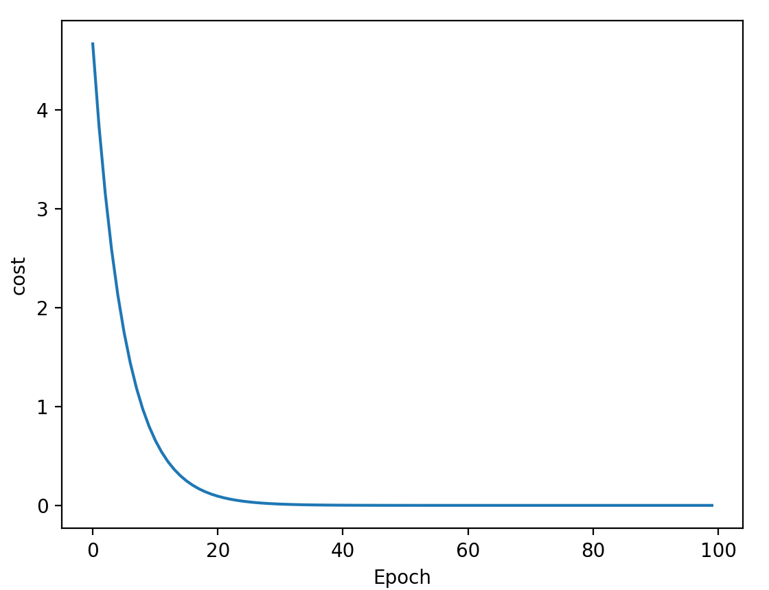
#梯度下降法
from matplotlib import pyplot as plt

# prepare the training set
x_data = [1.0, 2.0, 3.0]
y_data = [2.0, 4.0, 6.0]

# initial guess of weight
w = 1.0

# define the model linear model y = w*x
def forward(x):
    return x * w

#define the cost function MSE(均方差）
def cost(xs, ys):
    cost = 0
    for x, y in zip(xs, ys):
        y_pred = forward(x)
        cost += (y_pred - y) ** 2
    return cost / len(xs)

# define the gradient function  gd
def gradient(xs, ys):
    grad = 0
    for x, y in zip(xs, ys):
        grad += 2 * x * (x * w - y)
    return grad / len(xs)

epoch_list = []
cost_list = []
print('Predict (before training)', 4, forward(4))
for epoch in range(100):
    cost_val = cost(x_data, y_data)
    grad_val = gradient(x_data, y_data)
    w -= 0.01 * grad_val
    print('Epoch:', epoch, 'w=', w, 'loss=', cost_val)
    epoch_list.append(epoch)
    cost_list.append(cost_val)

print('Predict (after training)', 4, forward(4))
plt.plot(epoch_list, cost_list)
plt.xlabel('Epoch')
plt.ylabel('cost')
plt.show()

 

 

 

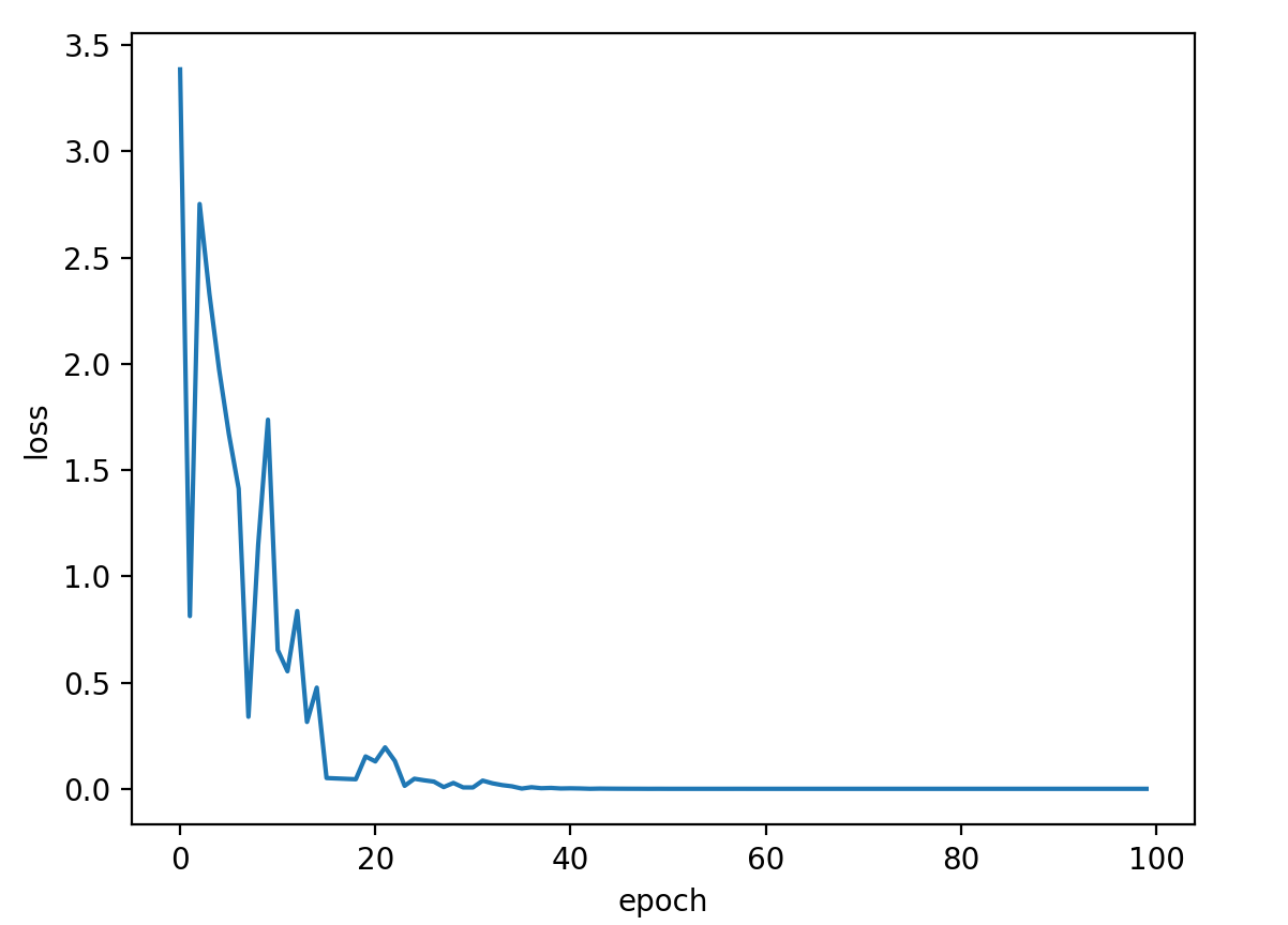
#随机梯度下降法,代码中没有体现哪里随机，差评，在网上找了一下随机怎么加，加了一个随机
'''随机梯度下降法在神经网络中被证明是有效的。效率较低(时间复杂度较高)，学习性能较好。
（梯度下降法计算时可以并行，所以效率好，但是容易进入鞍点；
随机梯度下降需要等待上一个值运行完才能更新下一个值，无法并行计算，但是某种程度上能解决鞍点问题；
因此，有种折中的办法叫batch。）

随机梯度下降法和梯度下降法的主要区别在于：
1、损失函数由cost()更改为loss()。cost是计算所有训练数据的损失，loss是计算一个训练函数的损失。对应于源代码则是少了两个for循环。
2、梯度函数gradient()由计算所有训练数据的梯度更改为计算一个训练数据的梯度。
'''
import random
import matplotlib.pyplot as plt

x_data = [1.0, 2.0, 3.0]
y_data = [2.0, 4.0, 6.0]

w = 1.0

def forward(x):
    return x * w

# calculate loss function
def loss(x, y):
    y_pred = forward(x)
    return (y_pred - y) ** 2

# define the gradient function  sgd（随机梯度下降）
def gradient(x, y):
    return 2 * x * (x * w - y)

epoch_list = []
loss_list = []
print('predict (before training)', 4, forward(4))
for epoch in range(100):
    #原代码
    # for x, y in zip(x_data, y_data):
    #     grad = gradient(x, y)
    #     w = w - 0.01 * grad  # update weight by every grad of sample of training set
    #     print("\tgrad:", x, y, grad)
    #     l = loss(x, y)
    # print("progress:", epoch, "w=", w, "loss=", l)
    #加随机
    rc = random.randrange(0,3)
    x1 = x_data[rc]
    y1 = y_data[rc]
    grad = gradient(x1, y1)
    w = w - 0.01 * grad
    l = loss(x1, y1)

    epoch_list.append(epoch)
    loss_list.append(l)

print('predict (after training)', 4, forward(4))
plt.plot(epoch_list, loss_list)
plt.ylabel('loss')
plt.xlabel('epoch')
plt.show()