Python数据分析与挖掘实战(5章)
非原创,仅个人关于《Python数据分析与挖掘实战》的学习笔记
5 挖掘建模
import warnings
import matplotlib.pyplot as plt
import numpy as np
import pandas as pd
# 解决中文乱码
plt.rcParams['font.sans-serif'] = ['SimHei']
plt.rcParams['axes.unicode_minus'] = False
# 忽略警告
warnings.filterwarnings("ignore")
5.1 分类与预测
5.1.1 实现过程
分类
分类是构造一个分类模型,输入样本的属性值,输出对应的类别,将每个样本映射到预先定义好的类别。分类属于有监督的学习。
- 1、学习,通过归纳分析训练样本集,建立分类模型,得到分类规则;
- 2、分类,先用已知的测试样本集评估分类规则的准确率,如果准确率可接受,则使用该模型对未分类的待测样本进行分类。
预测
预测是指建立两种或两种以上变量间相互依赖的函数模型,然后进行预测或控制。
- 1、通过训练集建立预测属性的函数模型
- 2、在模型通过检验后进行预测或控制
5.1.2 常用的分类与预测算法
回归分析
- 线性回归
- 非线性回归
- 逻辑回归
- 岭回归
- 主成分回归
- 偏最小二乘回归
决策树
自顶向下的递归方式,在颞部节点进行属性值的比较,并根据不同的属性值从该节点向下分支,最终得到的叶节点是学习划分的类。
贝叶斯
目前不确定知识表达和推理领域最有效的理论模型之一。
SVM
强大的模型,可以用来回归、预测、分类等,而根据选取不同的核函数。模型可以是线性的/非线性的。
随机森林
精度高于决策树,缺点是随机性,丧失了决策树的可解释性。
5.1.3 回归分析
import pandas as pd
from io import StringIO

# 手动转换图片中的数据为CSV格式
data = """年龄,教育,工龄,地址,收入,负债率,信用卡负债,其他负债,违约
41,3,17,12,176.00,9.30,11.36,5.01,1
27,1,10,6,31.00,17.30,1.36,4.00,0
40,1,15,14,55.00,5.50,0.86,2.17,0
41,1,15,14,120.00,2.90,2.66,0.82,0
24,2,2,0,28.00,17.30,1.79,3.06,1
"""

# 使用pandas读取CSV数据
df = pd.read_csv(StringIO(data))

# 显示DataFrame
df
| 年龄 | 教育 | 工龄 | 地址 | 收入 | 负债率 | 信用卡负债 | 其他负债 | 违约 | |
|---|---|---|---|---|---|---|---|---|---|
| 0 | 41 | 3 | 17 | 12 | 176.0 | 9.3 | 11.36 | 5.01 | 1 |
| 1 | 27 | 1 | 10 | 6 | 31.0 | 17.3 | 1.36 | 4.00 | 0 |
| 2 | 40 | 1 | 15 | 14 | 55.0 | 5.5 | 0.86 | 2.17 | 0 |
| 3 | 41 | 1 | 15 | 14 | 120.0 | 2.9 | 2.66 | 0.82 | 0 |
| 4 | 24 | 2 | 2 | 0 | 28.0 | 17.3 | 1.79 | 3.06 | 1 |
逻辑回归(Logistic)
import pandas as pd
import numpy as np
from io import StringIO
from sklearn.model_selection import train_test_split
from sklearn.linear_model import LogisticRegression
from sklearn.feature_selection import SelectFromModel
from sklearn.metrics import classification_report, accuracy_score
# 示例数据
data = """年龄,教育,工龄,地址,收入,负债率,信用卡负债,其他负债,违约
41,3,17,12,176.00,9.30,11.36,5.01,1
27,1,10,6,31.00,17.30,1.36,4.00,0
40,1,15,14,55.00,5.50,0.86,2.17,0
41,1,15,14,120.00,2.90,2.66,0.82,0
24,2,2,0,28.00,17.30,1.79,3.06,1
"""

# 使用pandas读取CSV数据
df = pd.read_csv(StringIO(data))

# 设置随机种子
np.random.seed(42)

# 生成100条新数据
new_data = {
    '年龄': np.random.randint(20, 60, 100),
    '教育': np.random.randint(1, 5, 100),
    '工龄': np.random.randint(1, 35, 100),
    '地址': np.random.randint(0, 20, 100),
    '收入': np.random.uniform(20.0, 200.0, 100),
    '负债率': np.random.uniform(1.0, 20.0, 100),
    '信用卡负债': np.random.uniform(0.5, 15.0, 100),
    '其他负债': np.random.uniform(0.1, 10.0, 100),
    '违约': np.random.randint(0, 2, 100)
}

new_df = pd.DataFrame(new_data)

# 合并数据
df = pd.concat([df, new_df], ignore_index=True)

# 定义特征和目标变量
X = df.drop(columns='违约')
y = df['违约']
X
| 年龄 | 教育 | 工龄 | 地址 | 收入 | 负债率 | 信用卡负债 | 其他负债 | |
|---|---|---|---|---|---|---|---|---|
| 0 | 41 | 3 | 17 | 12 | 176.000000 | 9.300000 | 11.360000 | 5.010000 |
| 1 | 27 | 1 | 10 | 6 | 31.000000 | 17.300000 | 1.360000 | 4.000000 |
| 2 | 40 | 1 | 15 | 14 | 55.000000 | 5.500000 | 0.860000 | 2.170000 |
| 3 | 41 | 1 | 15 | 14 | 120.000000 | 2.900000 | 2.660000 | 0.820000 |
| 4 | 24 | 2 | 2 | 0 | 28.000000 | 17.300000 | 1.790000 | 3.060000 |
| ... | ... | ... | ... | ... | ... | ... | ... | ... |
| 100 | 28 | 2 | 30 | 7 | 160.633289 | 15.241988 | 14.800726 | 2.129518 |
| 101 | 27 | 1 | 8 | 12 | 40.423628 | 8.466800 | 8.280564 | 3.854363 |
| 102 | 31 | 1 | 27 | 0 | 187.567239 | 16.754120 | 13.898606 | 9.271849 |
| 103 | 53 | 3 | 27 | 15 | 195.364678 | 11.812548 | 3.923690 | 7.243806 |
| 104 | 52 | 2 | 34 | 6 | 199.267624 | 2.206725 | 11.519353 | 0.576137 |
105 rows × 8 columns
y
0      1
1      0
2      0
3      0
4      1
      ..
100    1
101    0
102    0
103    1
104    0
Name: 违约, Length: 105, dtype: int64
# 拆分训练集和测试集
X_train, X_test, y_train, y_test = train_test_split(X, y, test_size=0.2, random_state=42)

# 使用随机逻辑回归模型筛选变量
sel = SelectFromModel(LogisticRegression(random_state=42, solver='liblinear'))
sel.fit(X_train, y_train)

# 获取被选中的特征
selected_features = X.columns[sel.get_support()]

# 训练逻辑回归模型
model = LogisticRegression(random_state=42, solver='liblinear')
model.fit(X_train[selected_features], y_train)

# 预测测试集
y_pred = model.predict(X_test[selected_features])

# 计算并保留训练集上的模型得分
train_score = model.score(X_train[selected_features], y_train)
train_score = f"{train_score:.2f}"
print(f"选中的特征: {selected_features}")
print(f"模型准确率: {train_score}")
选中的特征: Index(['地址', '其他负债'], dtype='object')
模型准确率: 0.67
简单例子
from sklearn.linear_model import LogisticRegression
from sklearn.model_selection import train_test_split
from sklearn.metrics import accuracy_score

# 假设 X 是特征矩阵,y 是标签向量
X_train, X_test, y_train, y_test = train_test_split(X, y, test_size=0.2, random_state=42)

# 创建逻辑回归模型
model = LogisticRegression()

# 训练模型
model.fit(X_train, y_train)

# 进行预测
y_pred = model.predict(X_test)

# 计算准确率
accuracy = accuracy_score(y_test, y_pred)
print(f"准确率: {accuracy}")
准确率: 0.6190476190476191
5.1.2 决策树
from sklearn.datasets import make_classification
from sklearn.model_selection import train_test_split
from sklearn.tree import DecisionTreeClassifier
from sklearn.metrics import accuracy_score
from sklearn import tree

# n_samples: 数据集中的样本数量。
# n_features: 数据集中的特征(变量)数量。
# n_informative: 对类别有影响的信息性特征的数量。
# n_redundant: 完全冗余的特征的数量(即可以由其他特征完全预测的特征)。
# n_repeated: 重复特征的数量。
# n_classes: 数据集中的类别数量。
# n_clusters_per_class: 每个类别中簇的数量。
# weights: 每个类别的权重。
# flip_y: 标签翻转的概率,用于引入噪声。
# random_state: 随机状态的种子,用于确保结果的可重复性。

# 创建一个合成数据集,这里我们使用scikit-learn内置的make_classification函数来生成
# 假设我们有以下特征:年龄、体重、经验(初学者、中级、高级)、健康状况(好、一般、差)
X, y = make_classification(n_samples=1000, n_features=4, n_informative=2, n_redundant=0, random_state=42)

# 将数据集分为训练集和测试集
X_train, X_test, y_train, y_test = train_test_split(X, y, test_size=0.2, random_state=42)

# 创建决策树分类器实例
clf = DecisionTreeClassifier()

# 训练模型
clf.fit(X_train, y_train)

# 对测试集进行预测
y_pred = clf.predict(X_test)

# 计算准确率
accuracy = accuracy_score(y_test, y_pred)
print(f"模型准确率: {accuracy:.2f}")

# 预测新的例子
# 假设我们有一个新的例子:年龄30,体重70公斤,经验中级,健康状况好
new_example = [[30, 70, 1, 0]]  # 特征编码:年龄, 体重, 经验(中级=1, 其他=0),健康状况(好=0, 其他=1)
print("新例子是否适合爬山: ", "适合" if clf.predict(new_example)[0] == 1 else "不适合")
模型准确率: 0.89
新例子是否适合爬山:  不适合
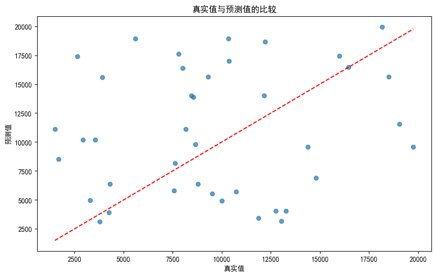
使用决策树模型预测销量
import pandas as pd
import numpy as np
from sklearn.model_selection import train_test_split
from sklearn.tree import DecisionTreeRegressor
from sklearn.metrics import mean_squared_error, r2_score
import matplotlib.pyplot as plt

# 生成示例数据
np.random.seed(42)
data = {
    '广告费用': np.random.uniform(1000, 5000, 200),
    '商店大小': np.random.uniform(50, 500, 200),
    '季节': np.random.choice(['春', '夏', '秋', '冬'], 200),
    '销量': np.random.uniform(1000, 20000, 200)
}

df = pd.DataFrame(data)

# 编码分类变量
df = pd.get_dummies(df, columns=['季节'], drop_first=True)

# 定义特征和目标变量
X = df.drop(columns='销量')
y = df['销量']

# 拆分数据集
X_train, X_test, y_train, y_test = train_test_split(X, y, test_size=0.2, random_state=42)

# 训练决策树回归模型
model = DecisionTreeRegressor(random_state=42)
model.fit(X_train, y_train)

# 预测
y_pred = model.predict(X_test)

# 评估模型
mse = mean_squared_error(y_test, y_pred)
r2 = r2_score(y_test, y_pred)

print(f"均方误差: {mse:.2f}")
print(f"拟合度: {r2:.2f}")

# 可视化真实值与预测值
plt.figure(figsize=(10, 6))
plt.scatter(y_test, y_pred, alpha=0.7)
plt.xlabel("真实值")
plt.ylabel("预测值")
plt.title("真实值与预测值的比较")
plt.plot([min(y_test), max(y_test)], [min(y_test), max(y_test)], 'r--')
plt.show()
均方误差: 46978560.88
拟合度: -0.89
df
| 广告费用 | 商店大小 | 销量 | 季节_夏 | 季节_春 | 季节_秋 | |
|---|---|---|---|---|---|---|
| 0 | 2498.160475 | 338.914241 | 14265.072566 | False | True | False |
| 1 | 4802.857226 | 87.862984 | 11185.830961 | True | False | False |
| 2 | 3927.975767 | 122.732921 | 6881.024709 | False | True | False |
| 3 | 3394.633937 | 454.349385 | 16462.105374 | False | True | False |
| 4 | 1624.074562 | 322.893077 | 14009.892279 | True | False | False |
| ... | ... | ... | ... | ... | ... | ... |
| 195 | 2396.838298 | 468.840797 | 12601.780806 | False | True | False |
| 196 | 3903.822715 | 436.285738 | 6483.980512 | False | True | False |
| 197 | 4588.441040 | 243.047312 | 12043.526207 | False | False | False |
| 198 | 4548.345697 | 387.891981 | 3932.891590 | False | False | False |
| 199 | 4119.502183 | 389.544293 | 10141.661935 | False | False | True |
200 rows × 6 columns
5.1.3 神经网络
# 人工神经元模型
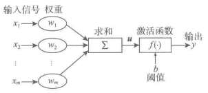
# 人工神经网络的学习=>训练(fit)
什么叫训练?
是指神经网络在受到外部环境的刺激下调整神经网络的参数,使神经网络以一种新的方式对外部环境作出反应的一个过程。
激活函数是什么?
1.域值函数
2.分段线性函数(Tanh (Hyperbolic Tangent))
# 将输入压缩到-1和1之间,比Sigmoid有更宽的输出范围。
3.非线性转移函数(Sigmoid)
# 将输入压缩到0和1之间,通常用于二分类问题。
4.Relu函数
# 当输入大于0时输出输入值,否则输出0。它计算简单,训练速度快,是目前最流行的激活函数之一。
5.PReLU
# Leaky ReLU的泛化形式,其中𝛼是可学习的参数。
6.Softmax
# 将输入的向量转换为概率分布,通常用于多分类问题的输出层。
7.ELU (Exponential Linear Unit)
# 对于负值,输出一个小于零的值,有助于缓解神经元的死亡问题。
实际案例
import numpy as np
import pandas as pd

# 加载数据
df = pd.read_csv('data/housing.csv')
df.describe()
| longitude | latitude | housing_median_age | total_rooms | total_bedrooms | population | households | median_income | median_house_value | |
|---|---|---|---|---|---|---|---|---|---|
| count | 20640.000000 | 20640.000000 | 20640.000000 | 20640.000000 | 20433.000000 | 20640.000000 | 20640.000000 | 20640.000000 | 20640.000000 |
| mean | -119.569704 | 35.631861 | 28.639486 | 2635.763081 | 537.870553 | 1425.476744 | 499.539680 | 3.870671 | 206855.816909 |
| std | 2.003532 | 2.135952 | 12.585558 | 2181.615252 | 421.385070 | 1132.462122 | 382.329753 | 1.899822 | 115395.615874 |
| min | -124.350000 | 32.540000 | 1.000000 | 2.000000 | 1.000000 | 3.000000 | 1.000000 | 0.499900 | 14999.000000 |
| 25% | -121.800000 | 33.930000 | 18.000000 | 1447.750000 | 296.000000 | 787.000000 | 280.000000 | 2.563400 | 119600.000000 |
| 50% | -118.490000 | 34.260000 | 29.000000 | 2127.000000 | 435.000000 | 1166.000000 | 409.000000 | 3.534800 | 179700.000000 |
| 75% | -118.010000 | 37.710000 | 37.000000 | 3148.000000 | 647.000000 | 1725.000000 | 605.000000 | 4.743250 | 264725.000000 |
| max | -114.310000 | 41.950000 | 52.000000 | 39320.000000 | 6445.000000 | 35682.000000 | 6082.000000 | 15.000100 | 500001.000000 |
5.2 聚类分析
5.2.1 K-Means聚类
- 这是最常用的聚类算法之一。首先随机选择K个中心点,然后将每个样本分配给最近的中心点,形成K个簇。
- 更新中心点为每个簇内所有点的均值,然后重复分配和更新过程,直到收敛。
5.2.2 层次聚类(Hierarchical Clustering)
- 层次聚类通过逐步合并或分裂样本来构建一个层次嵌套的簇树(树状层次结构)。
- 有两种主要的方法:凝聚的(自底向上)和分裂的(自顶向下)。
5.2.3 DBSCAN 基于密度的聚类算法
- DBSCAN基于密度的聚类算法,可以发现任意形状的簇,并且对噪声点具有鲁棒性。
- 它通过在高密度区域找到核心点,并将这些点及其邻域中的其他点合并到同一个簇。
5.2.4 Mean Shift聚类
- Mean Shift是一种基于密度的非参数聚类算法,它通过寻找密度函数的局部极大值点来确定簇中心。
它不需要事先指定簇的数量,而是根据数据的密度来自然形成簇。
5.2.5 谱聚类(Spectral Clustering)
谱聚类使用数据的相似性矩阵,通过将相似性矩阵转换为一组特征向量和特征值来发现数据的低维表示。
然后基于这些特征向量进行聚类。
聚类分析的一般步骤:
1.选择聚类算法:根据数据的特性和分析的目标选择合适的聚类算法。
2.准备数据:对数据进行预处理,如标准化、去除噪声等。
3.确定簇的数量:对于某些算法(如K-Means),需要预先指定簇的数量。
4.执行聚类:运行聚类算法,对数据进行分组。
5.评估聚类效果:使用轮廓系数、戴维森堡丁指数等指标评估聚类效果。
6.解释结果:根据聚类结果进行分析,解释簇的意义。
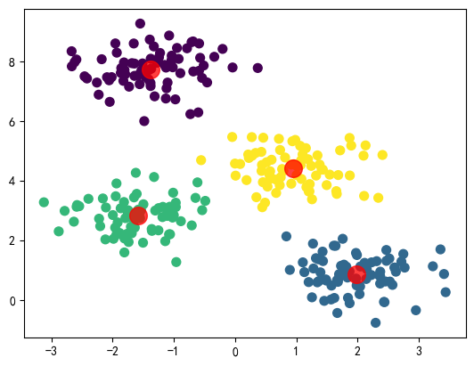
使用K-Means聚类
from sklearn.cluster import KMeans
from sklearn.datasets import make_blobs
import matplotlib.pyplot as plt

# 生成模拟数据
X, y = make_blobs(n_samples=300, centers=4, cluster_std=0.60, random_state=0)

# 执行K-Means聚类
kmeans = KMeans(n_clusters=4)
kmeans.fit(X)
predicted_labels = kmeans.predict(X)

# 可视化聚类结果
plt.scatter(X[:, 0], X[:, 1], c=predicted_labels, s=50, cmap='viridis')
centers = kmeans.cluster_centers_
plt.scatter(centers[:, 0], centers[:, 1], c='red', s=200, alpha=0.75)
plt.show()
import pandas as pd
from sklearn.datasets import make_blobs

# 生成模拟数据,默认情况下make_blobs生成的数据是两个特征的
X, y = make_blobs(n_samples=300, centers=4, cluster_std=0.60, random_state=0)

# 将X转换为DataFrame,每个特征一列
df_X = pd.DataFrame(X, columns=['feature_1', 'feature_2'])

# 将y转换为Series
series_y = pd.Series(y, name='target')

# df = pd.concat([df_X, series_y], axis=1)
# df
import pandas as pd
from sklearn.datasets import make_blobs
from sklearn.manifold import TSNE
import matplotlib.pyplot as plt
# 使用t-SNE降维
tsne = TSNE(n_components=2, random_state=0)
tsne_results = tsne.fit_transform(df_X)

# 创建一个新的DataFrame来保存t-SNE结果
df_tsne = pd.DataFrame(tsne_results, columns=['t-SNE-1', 't-SNE-2'])
df_tsne['Cluster'] = series_y  # 将原始的聚类标签添加到t-SNE结果中

# 绘制聚类效果图
plt.figure(figsize=(10, 8))
for cluster in df['target'].unique():
    cluster_data = df_tsne[df_tsne['Cluster'] == cluster]
    plt.scatter(cluster_data['t-SNE-1'], cluster_data['t-SNE-2'], label=f'Cluster {cluster}')
plt.title('t-SNE Visualization of Clusters')
plt.xlabel('t-SNE-1')
plt.ylabel('t-SNE-2')
plt.legend()
plt.show()

5.3 关联规则
# 关联规则分析,也叫购物篮分析。
# 用户买了面包,可能就会买牛奶。面包=>牛奶。
常用关联规则算法
Apriori算法
最常用、最经典,核心思想是通过连接产生候选项及其支持度然后通过剪枝生产频繁项集。
# 导入必要的库
from mlxtend.preprocessing import TransactionEncoder
from mlxtend.frequent_patterns import apriori, association_rules
import pandas as pd

# 定义一个商品购买记录的数据集,每个列表代表一个交易记录
dataset = [
    ['牛奶', '面包', '尿布'],
    ['可乐', '面包', '尿布', '啤酒'],
    ['牛奶', '尿布', '啤酒', '鸡蛋'],
    ['面包', '牛奶', '尿布'],
    ['面包', '牛奶', '尿布', '可乐', '啤酒'],
    ['尿布', '啤酒', '鸡蛋'],
    ['牛奶', '面包', '尿布', '鸡蛋']
]

# 使用TransactionEncoder转换交易数据集,使其适合机器学习模型处理
te = TransactionEncoder()

# fit()方法将数据集转换为one-hot编码形式
te_ary = te.fit(dataset).transform(dataset)

# transform()方法将转换后的数据集转换为DataFrame格式
df = pd.DataFrame(te_ary, columns=te.columns_)

# 使用apriori函数找出频繁项集
# min_support参数定义了项集出现的最小支持度(即在所有交易记录中出现的最小比例)
frequent_itemsets = apriori(df, min_support=0.5, use_colnames=True)
# 输出频繁项集的DataFrame
frequent_itemsets
| support | itemsets | |
|---|---|---|
| 0 | 0.571429 | (啤酒) |
| 1 | 1.000000 | (尿布) |
| 2 | 0.714286 | (牛奶) |
| 3 | 0.714286 | (面包) |
| 4 | 0.571429 | (啤酒, 尿布) |
| 5 | 0.714286 | (牛奶, 尿布) |
| 6 | 0.714286 | (尿布, 面包) |
| 7 | 0.571429 | (牛奶, 面包) |
| 8 | 0.571429 | (牛奶, 尿布, 面包) |
# 使用association_rules函数根据频繁项集生成关联规则
# metric="confidence"表示使用置信度作为衡量规则强度的指标
# min_threshold=0.7定义了最小置信度阈值
rules = association_rules(frequent_itemsets, metric="confidence", min_threshold=0.7)
# 输出关联规则的DataFrame
rules
| antecedents | consequents | antecedent support | consequent support | support | confidence | lift | leverage | conviction | zhangs_metric | |
|---|---|---|---|---|---|---|---|---|---|---|
| 0 | (啤酒) | (尿布) | 0.571429 | 1.000000 | 0.571429 | 1.000000 | 1.00 | 0.000000 | inf | 0.000 |
| 1 | (牛奶) | (尿布) | 0.714286 | 1.000000 | 0.714286 | 1.000000 | 1.00 | 0.000000 | inf | 0.000 |
| 2 | (尿布) | (牛奶) | 1.000000 | 0.714286 | 0.714286 | 0.714286 | 1.00 | 0.000000 | 1.000000 | 0.000 |
| 3 | (尿布) | (面包) | 1.000000 | 0.714286 | 0.714286 | 0.714286 | 1.00 | 0.000000 | 1.000000 | 0.000 |
| 4 | (面包) | (尿布) | 0.714286 | 1.000000 | 0.714286 | 1.000000 | 1.00 | 0.000000 | inf | 0.000 |
| 5 | (牛奶) | (面包) | 0.714286 | 0.714286 | 0.571429 | 0.800000 | 1.12 | 0.061224 | 1.428571 | 0.375 |
| 6 | (面包) | (牛奶) | 0.714286 | 0.714286 | 0.571429 | 0.800000 | 1.12 | 0.061224 | 1.428571 | 0.375 |
| 7 | (牛奶, 尿布) | (面包) | 0.714286 | 0.714286 | 0.571429 | 0.800000 | 1.12 | 0.061224 | 1.428571 | 0.375 |
| 8 | (牛奶, 面包) | (尿布) | 0.571429 | 1.000000 | 0.571429 | 1.000000 | 1.00 | 0.000000 | inf | 0.000 |
| 9 | (尿布, 面包) | (牛奶) | 0.714286 | 0.714286 | 0.571429 | 0.800000 | 1.12 | 0.061224 | 1.428571 | 0.375 |
| 10 | (牛奶) | (尿布, 面包) | 0.714286 | 0.714286 | 0.571429 | 0.800000 | 1.12 | 0.061224 | 1.428571 | 0.375 |
| 11 | (面包) | (牛奶, 尿布) | 0.714286 | 0.714286 | 0.571429 | 0.800000 | 1.12 | 0.061224 | 1.428571 | 0.375 |
解释第一条:
用户同时买啤酒喝尿布的概率是57.14%,买了啤酒,再买尿布的概率是100%。
5.4 时序模式
基于给定的一个已被观测了的时间序列,预测该序列的未来值。
5.4.1 时间序列算法
常用事件序列模型算法:
- 1.平滑法
- 2.趋势拟合法
- 3.组合模型
- 4.AR模型
- 5.MA模型
- 6.ARMA模型
- 7.ARIMA模型
- 8.ARCH模型
- 9.GARCH模型及其衍生模型
5.4.2 时间序列的预处理
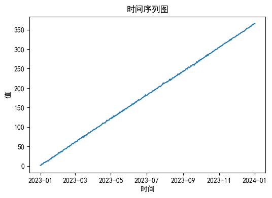
5.4.2.1 平稳性检验
# 时序图检验案例
import pandas as pd
import numpy as np
import matplotlib.pyplot as plt

# 设置随机种子以获得可重复的结果
np.random.seed(42)

# 创建时间序列的时间索引
start_date = pd.Timestamp('2023-01-01')
end_date = pd.Timestamp('2024-01-01')
time_index = pd.date_range(start_date, end_date, freq='D')

# 生成随机时间序列数据
# 趋势成分:线性增长
trend = np.arange(1, len(time_index) + 1)
# 季节性成分:周期性变化
seasonality = np.sin(2 * np.pi * time_index.dayofyear / 365)
# 随机噪声:随机波动
noise = np.random.normal(0, 1, len(time_index))
# 时间序列 = 趋势 + 季节性成分 + 随机噪声
data = trend + seasonality + noise

# 创建DataFrame
df = pd.DataFrame(data, index=time_index, columns=['Value'])

# # 绘制时间序列图
# plt.figure(figsize=(12, 6))
# plt.plot(df.index, df['Value'], label='Time Series')
# plt.title('Random Time Series Data')
# plt.xlabel('Date')
# plt.ylabel('Value')
# plt.legend()
# plt.show()

# 输出生成的数据
df
| Value | |
|---|---|
| 2023-01-01 | 1.513928 |
| 2023-01-02 | 1.896157 |
| 2023-01-03 | 3.699308 |
| 2023-01-04 | 5.591832 |
| 2023-01-05 | 4.851811 |
| ... | ... |
| 2023-12-28 | 363.481119 |
| 2023-12-29 | 362.856818 |
| 2023-12-30 | 364.384498 |
| 2023-12-31 | 365.690144 |
| 2024-01-01 | 365.615993 |
366 rows × 1 columns
import matplotlib.pyplot as plt
import pandas as pd

# 绘制时序图
plt.figure(figsize=(6, 4))
plt.plot(df.index, df.values)  # 使用.values来获取数据值
plt.title('时间序列图')
plt.xlabel('时间')
plt.ylabel('值')
plt.show()
# 自相关图检验案例
import pandas as pd
import numpy as np
import matplotlib.pyplot as plt
from statsmodels.graphics.tsaplots import plot_acf, plot_pacf
# 继续使用上面的df数据
# 绘制自相关图
plot_acf(df)
plt.title('自相关图')
plt.show()
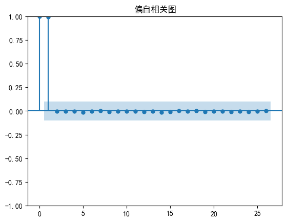
# 绘制偏自相关图
plot_pacf(df)
plt.title('偏自相关图')
plt.show()

# 单位根检验案例
from statsmodels.tsa.stattools import adfuller

# 对时间序列进行ADF检验
result = adfuller(df, autolag='AIC')  # AIC用于选择滞后阶数

# 输出检验结果
print('ADF检验结果:')
print(f'ADF统计量: {result[0]}')
print(f'p值: {result[1]}')
print('临界值:')
for key, value in result[4].items():
    print(f'{key}: {value}')
ADF检验结果:
ADF统计量: 0.37414128225640897
p值: 0.9805017342351662
临界值:
1%: -3.448905534655263
5%: -2.8697161816205705
10%: -2.5711258103550882
结论
p 值为 0.9805017342351662。由于 p 值大于 0.05 的显著性水平,所以不能拒绝原假设,即时间序列存在单位根,是非平稳的。
5.4.2.2 纯随机性检验
import pandas as pd
import numpy as np
from statsmodels.stats.diagnostic import acorr_ljungbox

def generate_random_data():
    # 生成随机时间序列数据
    np.random.seed(42)  # 设置随机种子以确保结果可重复
    date_range = pd.date_range(start='2023-01-01', end='2023-12-31', freq='D')  # 日期范围
    data = np.random.randn(len(date_range))  # 随机数据

    # 创建 DataFrame
    df = pd.DataFrame(data, index=date_range, columns=['Value'])

    return df

def test_white_noise(data):
    # 进行 Ljung-Box 检验
    lb_test = acorr_ljungbox(data['Value'], lags=10)  # lags 为 10

    # 从结果中提取检验统计量和 p 值
    test_stat = lb_test['lb_stat']
    p_values = lb_test['lb_pvalue']

    # 输出检验统计量和 p 值
    print("Ljung-Box 检验统计量:", test_stat)
    print("Ljung-Box 检验 p 值:", p_values)

    if len(test_stat) > 0:
        print("Ljung-Box 检验统计量:", test_stat)
    else:
        print("无法获取 Ljung-Box 检验统计量")

# 生成随机数据
data = generate_random_data()

# 调用纯随机性检验函数
test_white_noise(data)
Ljung-Box 检验统计量: 1      1.408778
2      1.582490
3      2.159862
4      5.583555
5      6.959789
6      8.233302
7      8.310180
8      8.862838
9      9.413086
10    10.089407
Name: lb_stat, dtype: float64
Ljung-Box 检验 p 值: 1     0.235259
2     0.453280
3     0.539898
4     0.232482
5     0.223648
6     0.221504
7     0.306039
8     0.353999
9     0.400049
10    0.432685
Name: lb_pvalue, dtype: float64
Ljung-Box 检验统计量: 1      1.408778
2      1.582490
3      2.159862
4      5.583555
5      6.959789
6      8.233302
7      8.310180
8      8.862838
9      9.413086
10    10.089407
Name: lb_stat, dtype: float64
5.4.3 平稳时间序列分析
5.4.4 非平稳时间序列分析
ARMA模型,自回归移动平均模型,目前最常用的拟合平稳序列的模型。细分:AR\MA\ARMA三大类。
import pandas as pd
import numpy as np
import matplotlib.pyplot as plt
# 设置随机种子以获得可重复的结果
np.random.seed(42)
# 创建时间序列的时间索引
start_date = pd.Timestamp('2023-01-01')
end_date = pd.Timestamp('2024-01-01')
time_index = pd.date_range(start_date, end_date, freq='D')
# 生成随机时间序列数据
# 趋势成分:线性增长
trend = np.arange(1, len(time_index) + 1)
# 季节性成分:周期性变化
seasonality = np.sin(2 * np.pi * time_index.dayofyear / 365)
# 随机噪声:随机波动
noise = np.random.normal(0, 1, len(time_index))
# 时间序列 = 趋势 + 季节性成分 + 随机噪声
data = trend + seasonality + noise
# 创建DataFrame
df = pd.DataFrame(data, index=time_index, columns=['Value'])
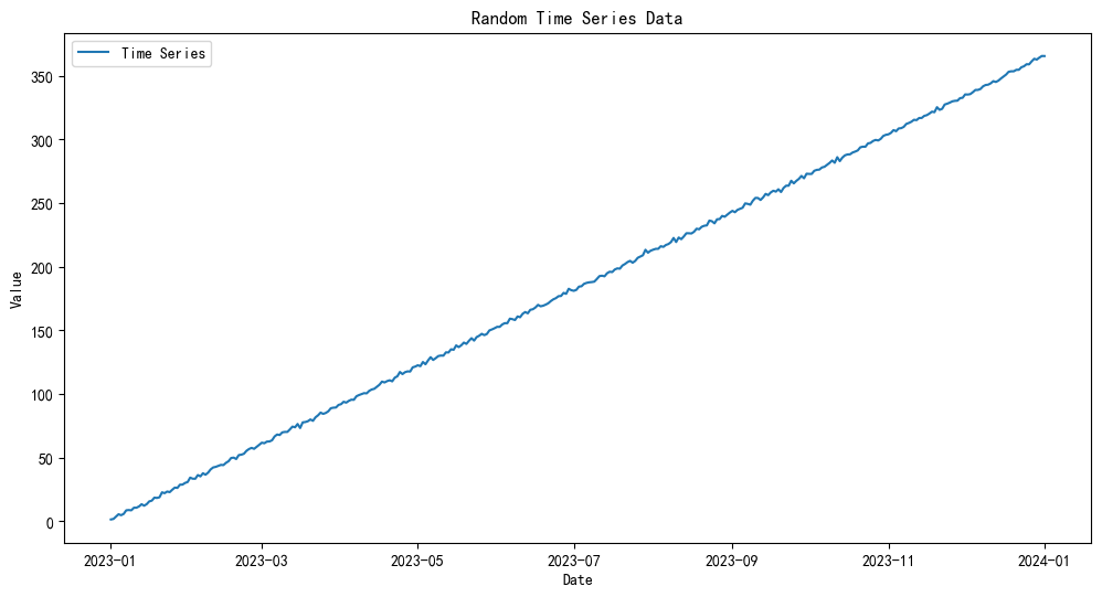
# 绘制时间序列图
plt.figure(figsize=(12, 6))
plt.plot(df.index, df['Value'], label='Time Series')
plt.title('Random Time Series Data')
plt.xlabel('Date')
plt.ylabel('Value')
plt.legend()
plt.show()
# 输出生成的数据
print(df.head())
               Value
2023-01-01  1.513928
2023-01-02  1.896157
2023-01-03  3.699308
2023-01-04  5.591832
2023-01-05  4.851811
AR模型
AR 模型是一种线性模型,它使用过去时间点的观测值来预测未来的观测值。AR 模型假设当前观测值是过去一段时间内的观测值的线性组合。
# 拟合 AR 模型
model_ar = ARIMA(df['Value'], order=(1, 0, 0))
results_ar = model_ar.fit()

# 打印模型摘要
print(results_ar.summary())

# 进行预测
forecast_ar = results_ar.forecast(steps=30)

# 绘制实际值和预测值
plt.figure(figsize=(10, 6))
plt.plot(df.index, df['Value'], label='Actual Values')
plt.plot(pd.date_range(start=df.index[-1] + pd.Timedelta(days=1), periods=30, freq='D'), forecast_ar, label='Forecast', color='red')
plt.title('AR Model Forecast')
plt.xlabel('Date')
plt.ylabel('Value')
plt.legend()
plt.show()
                               SARIMAX Results
==============================================================================
Dep. Variable:                  Value   No. Observations:                  366
Model:                 ARIMA(1, 0, 0)   Log Likelihood                -718.843
Date:                Mon, 27 May 2024   AIC                           1443.686
Time:                        11:48:00   BIC                           1455.394
Sample:                    01-01-2023   HQIC                          1448.338
                         - 01-01-2024
Covariance Type:                  opg
==============================================================================
                 coef    std err          z      P>|z|      [0.025      0.975]
------------------------------------------------------------------------------
const        183.5160    180.634      1.016      0.310    -170.520     537.552
ar.L1          1.0000      0.001   1105.416      0.000       0.998       1.002
sigma2         2.9000      0.247     11.735      0.000       2.416       3.384
===================================================================================
Ljung-Box (L1) (Q):                  96.11   Jarque-Bera (JB):                 2.47
Prob(Q):                              0.00   Prob(JB):                         0.29
Heteroskedasticity (H):               1.05   Skew:                            -0.20
Prob(H) (two-sided):                  0.77   Kurtosis:                         2.98
===================================================================================

Warnings:
[1] Covariance matrix calculated using the outer product of gradients (complex-step).

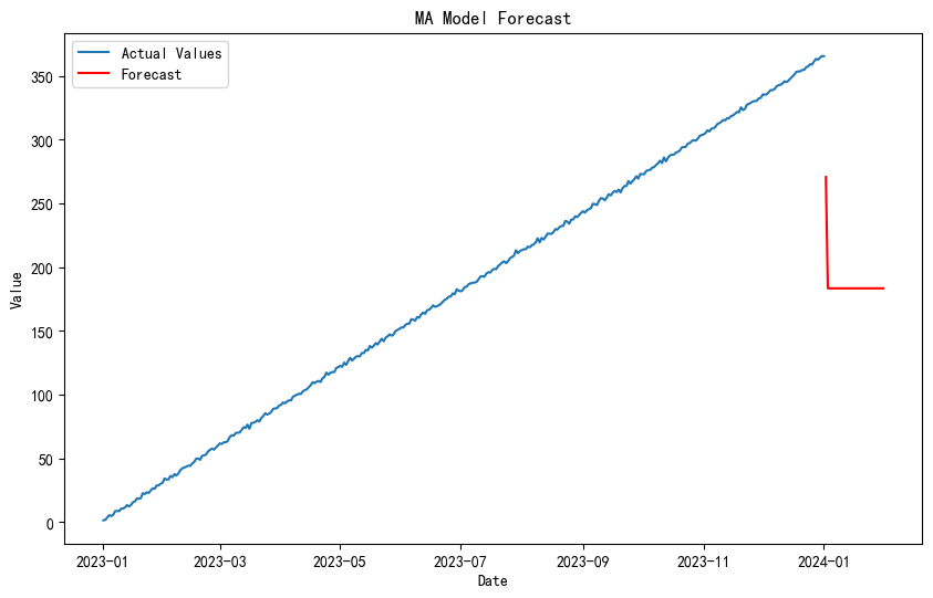
MA模型
MA 模型是一种线性模型,它使用过去时间点的随机误差来预测未来的观测值。MA 模型假设当前观测值是过去一段时间内的随机误差的加权和。
from statsmodels.tsa.arima.model import ARIMA

# 拟合 MA 模型
model_ma = ARIMA(df['Value'], order=(0, 0, 1))
results_ma = model_ma.fit()

# 打印模型摘要
print(results_ma.summary())

# 进行预测
forecast_ma = results_ma.forecast(steps=30)

# 绘制实际值和预测值
plt.figure(figsize=(10, 6))
plt.plot(df.index, df['Value'], label='Actual Values')
plt.plot(pd.date_range(start=df.index[-1] + pd.Timedelta(days=1), periods=30, freq='D'), forecast_ma, label='Forecast', color='red')
plt.title('MA Model Forecast')
plt.xlabel('Date')
plt.ylabel('Value')
plt.legend()
plt.show()
                               SARIMAX Results
==============================================================================
Dep. Variable:                  Value   No. Observations:                  366
Model:                 ARIMA(0, 0, 1)   Log Likelihood               -1977.279
Date:                Mon, 27 May 2024   AIC                           3960.559
Time:                        11:48:05   BIC                           3972.266
Sample:                    01-01-2023   HQIC                          3965.211
                         - 01-01-2024
Covariance Type:                  opg
==============================================================================
                 coef    std err          z      P>|z|      [0.025      0.975]
------------------------------------------------------------------------------
const        183.4987      5.519     33.247      0.000     172.681     194.316
ma.L1          0.9991      0.030     32.959      0.000       0.940       1.059
sigma2      2840.6270    341.058      8.329      0.000    2172.166    3509.088
===================================================================================
Ljung-Box (L1) (Q):                 332.66   Jarque-Bera (JB):                20.77
Prob(Q):                              0.00   Prob(JB):                         0.00
Heteroskedasticity (H):               1.01   Skew:                            -0.01
Prob(H) (two-sided):                  0.97   Kurtosis:                         1.83
===================================================================================

Warnings:
[1] Covariance matrix calculated using the outer product of gradients (complex-step).
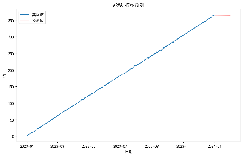
ARMA模型
ARMA 模型是 AR 和 MA 模型的组合,它同时考虑了过去观测值和过去随机误差来预测未来的观测值。
import pandas as pd
import numpy as np
import matplotlib.pyplot as plt
from statsmodels.tsa.arima.model import ARIMA
from statsmodels.graphics.tsaplots import plot_acf, plot_pacf

# 生成随机时间序列数据
np.random.seed(42)
start_date = pd.Timestamp('2023-01-01')
end_date = pd.Timestamp('2024-01-01')
time_index = pd.date_range(start_date, end_date, freq='D')
trend = np.arange(1, len(time_index) + 1)
seasonality = np.sin(2 * np.pi * time_index.dayofyear / 365)
noise = np.random.normal(0, 1, len(time_index))
data = trend + seasonality + noise
df = pd.DataFrame(data, index=time_index, columns=['Value'])

# 绘制时间序列图
plt.figure(figsize=(12, 6))
plt.plot(df.index, df['Value'], label='时间序列')
plt.title('随机时间序列数据')
plt.xlabel('日期')
plt.ylabel('值')
plt.legend()
plt.show()

# 计算 ACF 和 PACF
plot_acf(df['Value'], lags=40)
plt.title('自相关函数 (ACF)')
plt.xlabel('滞后')
plt.ylabel('ACF')
plt.show()

plot_pacf(df['Value'], lags=40)
plt.title('偏自相关函数 (PACF)')
plt.xlabel('滞后')
plt.ylabel('PACF')
plt.show()

# 拟合 ARMA 模型
model_arma = ARIMA(df['Value'], order=(2, 0, 1))
results_arma = model_arma.fit()

# 打印模型摘要
print(results_arma.summary())

# 进行预测
forecast_arma = results_arma.forecast(steps=30)

# 绘制实际值和预测值
plt.figure(figsize=(10, 6))
plt.plot(df.index, df['Value'], label='实际值')
plt.plot(pd.date_range(start=df.index[-1] + pd.Timedelta(days=1), periods=30, freq='D'), forecast_arma, label='预测值', color='red')
plt.title('ARMA 模型预测')
plt.xlabel('日期')
plt.ylabel('值')
plt.legend()
plt.show()


                               SARIMAX Results
==============================================================================
Dep. Variable:                  Value   No. Observations:                  366
Model:                 ARIMA(2, 0, 1)   Log Likelihood                -718.802
Date:                Mon, 27 May 2024   AIC                           1447.604
Time:                        12:03:18   BIC                           1467.118
Sample:                    01-01-2023   HQIC                          1455.358
                         - 01-01-2024
Covariance Type:                  opg
==============================================================================
                 coef    std err          z      P>|z|      [0.025      0.975]
------------------------------------------------------------------------------
const        183.5095    180.629      1.016      0.310    -170.517     537.537
ar.L1          0.0196      0.155      0.127      0.899      -0.284       0.323
ar.L2          0.9803      0.155      6.328      0.000       0.677       1.284
ma.L1          0.9774      0.166      5.901      0.000       0.653       1.302
sigma2         2.8994      0.249     11.628      0.000       2.411       3.388
===================================================================================
Ljung-Box (L1) (Q):                  95.26   Jarque-Bera (JB):                 2.42
Prob(Q):                              0.00   Prob(JB):                         0.30
Heteroskedasticity (H):               1.05   Skew:                            -0.20
Prob(H) (two-sided):                  0.79   Kurtosis:                         2.99
===================================================================================

Warnings:
[1] Covariance matrix calculated using the outer product of gradients (complex-step).
通过分析自相关函数(ACF)和偏自相关函数(PACF)图,可以帮助确定适合的模型阶数。例如,如果 ACF 在滞后阶数上衰减得很慢,而 PACF 在滞后阶数上截尾,可能是 AR 模型的候选。如果 ACF 和 PACF 都在滞后阶数上衰减得很慢,可能需要选择 ARMA 模型。
5.4.4 非平稳时间序列分析
- ARIMA模型
- 残差自回归模型
- 季节模型
- 异方差模型
ARIMA模型
- 1.读取数据并将其转换为时间序列格式。
- 2.绘制原始时间序列数据的时序图,以可视化其趋势和模式。
- 3.绘制原始时间序列数据的自相关图和偏自相关图,用于选择 ARIMA 模型的阶数。
- 4.进行平稳性检验,以确定是否需要对数据进行差分处理。
- 5.如果数据不平稳,进行一次差分,并再次绘制差分后数据的自相关图和偏自相关图。
- 6.再次进行平稳性检验,以确认差分后的数据是否满足平稳性要求。
- 7.根据选择的阶数构建了 ARIMA 模型,并进行拟合。
- 8.打印模型摘要,以查看模型的统计指标和参数估计值。
- 9.对模型进行诊断,包括残差的自相关性、残差的分布等。
import numpy as np
import matplotlib.pyplot as plt
from statsmodels.tsa.stattools import adfuller
from statsmodels.graphics.tsaplots import plot_acf, plot_pacf
from statsmodels.tsa.arima.model import ARIMA
from statsmodels.stats.diagnostic import acorr_ljungbox

# 读取数据
data = np.array([
    3023, 3039, 3056, 3138, 3188, 3224, 3226, 3029, 2859, 2870, 2910, 3012, 3012,
    3142, 3252, 3342, 3365, 3339, 3345, 3421, 3443, 3428, 3454, 3615, 3646, 3614, 3574, 3635, 3738,
    3707, 3827, 4039, 4210, 4493, 4560, 4637, 4755, 4817
])

# 将数据转换为时间序列格式
import pandas as pd
date = pd.date_range(start='2015-01-01', periods=len(data), freq='D')
ts = pd.Series(data, index=date)

# 绘制时序图
plt.figure(figsize=(12, 6))
plt.plot(ts, label='销量(元)')
plt.title('原时序图')
plt.legend()
plt.show()

# 自相关图和偏自相关图
plot_acf(ts)
plt.title('原始序列自相关图')
plt.show()
plot_pacf(ts)
plt.title('原始序列偏自相关图')
plt.show()

# 平稳性检测
# result = adfuller(ts)
# print('原始序列的ADF检验结果为: %f' % result[0])
# print('原始序列的p-value: %f' % result[1])
from statsmodels.tsa.stattools import adfuller as ADF
# print('原始序列的ADF检验结果为: %f \n',ADF(ts))
# print("返回值依次为:adf、pvalue、usedlag、nobs、critical values、icbest、regresults、resstore")

# 原始序列ADF检验结果(原始序列单位根检验)
adf_result = ADF(ts)

# 创建DataFrame对象
adf_df = pd.DataFrame({
    'adf': adf_result[0],
    'pvalue': adf_result[1],
    'usedlag': adf_result[2],
    'nobs': adf_result[3],
    'critical_values': adf_result[4],
    'icbest': adf_result[5]
})

# 白噪声检验
print(u'原始序列的白噪声检验结果是: \n', acorr_ljungbox(date, lags=1))


# 打印DataFrame对象(P值显著大于0.05,判断原序列为非平稳序列,非平稳序列一定不是白噪声序列)
print('平稳性检测结果:\n',adf_df)

# 如果数据不平稳,进行差分
if result[1] > 0.05:
    ts_diff = ts.diff().dropna()
    plt.figure(figsize=(12, 6))
    plt.plot(ts_diff, label='销量差分')
    plt.title('差分后的时序图')
    plt.legend()
    plt.show()

    # 再次绘制ACF和PACF
    plot_acf(ts_diff)
    plt.title('差分后的自相关图')
    plt.show()
    plot_pacf(ts_diff)
    plt.title('差分后的偏自相关图')
    plt.show()

    # 再次进行平稳性检测
    result_diff = adfuller(ts_diff)
    print('差分后序列的ADF检验结果为: %f' % result_diff[0])
    print('差分后序列的p-value: %f' % result_diff[1])

    # 白噪声检验
    print(u'差分序列的白噪声检验结果是: \n', acorr_ljungbox(ts_diff, lags=1))

# 定阶
# 根据ACF和PACF图选择p, d, q参数

# 假设我们选择了阶数 p=1, d=1, q=1
model = ARIMA(ts, order=(1, 1, 1))
model_fit = model.fit()

# 打印模型摘要
print(model_fit.summary())

# 模型诊断
model_fit.plot_diagnostics(figsize=(15, 12))
plt.show()


原始序列的白噪声检验结果是:
     lb_stat     lb_pvalue
1  34.85064  3.559925e-09
平稳性检测结果:
           adf    pvalue  usedlag  nobs  critical_values      icbest
1%   2.408377  0.999014        6    31        -3.661429  311.888583
10%  2.408377  0.999014        6    31        -2.619319  311.888583
5%   2.408377  0.999014        6    31        -2.960525  311.888583

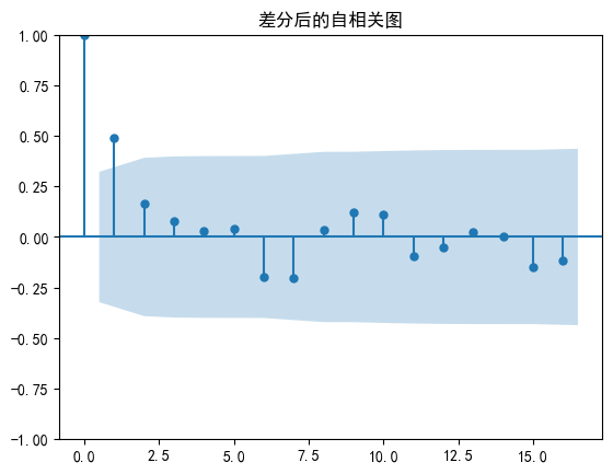

差分后序列的ADF检验结果为: -3.430178
差分后序列的p-value: 0.009972
差分序列的白噪声检验结果是:
     lb_stat  lb_pvalue
1  9.506743   0.002047
                               SARIMAX Results
==============================================================================
Dep. Variable:                      y   No. Observations:                   38
Model:                 ARIMA(1, 1, 1)   Log Likelihood                -215.075
Date:                Mon, 27 May 2024   AIC                            436.149
Time:                        16:07:57   BIC                            440.982
Sample:                    01-01-2015   HQIC                           437.853
                         - 02-07-2015
Covariance Type:                  opg
==============================================================================
                 coef    std err          z      P>|z|      [0.025      0.975]
------------------------------------------------------------------------------
ar.L1          0.5604      0.209      2.681      0.007       0.151       0.970
ma.L1          0.0484      0.277      0.175      0.861      -0.495       0.591
sigma2      6477.4981   1556.519      4.162      0.000    3426.776    9528.220
===================================================================================
Ljung-Box (L1) (Q):                   0.14   Jarque-Bera (JB):                 0.36
Prob(Q):                              0.71   Prob(JB):                         0.84
Heteroskedasticity (H):               1.62   Skew:                            -0.19
Prob(H) (two-sided):                  0.41   Kurtosis:                         3.29
===================================================================================

Warnings:
[1] Covariance matrix calculated using the outer product of gradients (complex-step).

# 预测未来一段时间的数据
forecast_steps = 7
forecast = model_fit.forecast(steps=forecast_steps)

# 将预测结果转换为时间序列格式
forecast_index = pd.date_range(start=ts.index[-1] + pd.Timedelta(days=1), periods=forecast_steps, freq='D')
forecast_series = pd.Series(forecast, index=forecast_index)

# 绘制原始数据和预测结果的时序图
plt.figure(figsize=(12, 6))
plt.plot(ts, label='原始')
plt.plot(forecast_series, label='预测', color='red')
plt.title('原始数据序列图及预测分析')
plt.legend()
plt.show()

主要时序模式算法:
- acf() #计算自相关系数
- plot_acf() #画自相关系数图
- pacf() #计算偏相关系数
- plot_pacf() #画偏相关系数图
- adfuller() #对观测值序列进行单位根检验
- diff() #对观测值序列进行差分计算
- ARIMA() #创建一个ARIMA时序模型
- summary()或summaty2 #给出一份ARIMA模型的报告
- aic/bic/hqic #计算ARIMA模型的AIC\BIC\HQIC指标值
- forecast() #应用构建的时序模型进行预测
- acorr_ljungbox() #Ljung-Box检验,检验是否为白噪声。
5.5 离群点检测
# 如何根据客户的消费记录检测是否为异常刷卡消费?
# 如何检测是否有异常订单?
# 可以通过离群点检测来解决这些问题。
离群点检测,也叫偏差检测,任务是发现与大部分其他对象显著不同的对象。
主要应用于信用卡检测、贷款审批、电子商务、网络入侵和天气预报等领域。
5.5.1 基于模型的离群点检测方法
5.5.1.1 一元正态分布中的离群点检测
- 将数据转换为时间序列格式。
- 计算时间序列的均值和标准差。
- 定义离群点的阈值(这里使用3个标准差)。
- 找出超过阈值的离群点。
- 绘制时序图并标记出离群点、均值以及阈值上下限。
- 打印出离群点。
import numpy as np
import pandas as pd
import matplotlib.pyplot as plt

# 读取数据
data = np.array([
    3023, 3039, 3056, 3138, 3188, 3224, 3226, 3029, 2859, 2870, 2910, 3012, 3012,
    3142, 3252, 3342, 3365, 1000, 3345, 3421, 3443, 3428, 3454, 3615, 3646, 3614, 3574, 3635, 3738,
    3707, 3827, 4039, 4210, 6000, 4560, 4637, 4755, 4817
])

# 将数据转换为时间序列格式
date = pd.date_range(start='2015-01-01', periods=len(data), freq='D')
ts = pd.Series(data, index=date)

# 计算均值和标准差
mean = ts.mean()
std = ts.std()

# 定义离群点的阈值(通常使用3个标准差)
threshold = 3

# 找出离群点
outliers = ts[np.abs((ts - mean) / std) > threshold]

# 绘制时序图和离群点
plt.figure(figsize=(12, 6))
plt.plot(ts, label='原数据')
plt.scatter(outliers.index, outliers, color='red', label='离群点')
plt.axhline(mean, color='green', linestyle='--', label='均值')
plt.axhline(mean + threshold * std, color='orange', linestyle='--', label='上限')
plt.axhline(mean - threshold * std, color='orange', linestyle='--', label='下限')
plt.title('基于一元正态分布的离群点检测')
plt.legend()
plt.show()

# 打印离群点
print("离群点如下:")
print(outliers)

离群点如下:
2015-01-18    1000
2015-02-03    6000
dtype: int32
5.5.1.2 混合模型的离群点检测
混合模型(Mixture Model)是一种统计模型,其中数据由多个分布组成。
常见的混合模型是高斯混合模型(Gaussian Mixture Model, GMM),用于表示由多个高斯分布组成的数据集。在时间序列分析中,可以使用GMM来检测离群点,因为GMM能够识别不同的数据模式,并将不符合任何模式的数据点标记为离群点。
- 将数据转换为时间序列格式。
- 对数据进行标准化处理,使其均值为0,标准差为1。
- 将数据转换为适合GMM的二维数组。
- 拟合GMM模型,选择2个高斯成分(可以根据实际情况调整)。
- 计算每个数据点的异常得分(负对数概率)。
- 使用95百分位数作为阈值来识别离群点。
- 绘制时序图并标记出离群点.
- 打印出离群点。
import numpy as np
import pandas as pd
import matplotlib.pyplot as plt
from sklearn.mixture import GaussianMixture

# 读取数据
data = np.array([
    3023, 3039, 3056, 3138, 3188, 3224, 3226, 3029, 2859, 2870, 2910, 3012, 3012,
    3142, 3252, 3342, 3365, 3339, 3345, 3421, 3443, 3428, 3454, 3615, 3646, 3614, 3574, 3635, 3738,
    3707, 3827, 4039, 4210, 4493, 4560, 4637, 4755, 4817
])

# 将数据转换为时间序列格式
date = pd.date_range(start='2015-01-01', periods=len(data), freq='D')
ts = pd.Series(data, index=date)

# 数据标准化
ts_mean = ts.mean()
ts_std = ts.std()
ts_normalized = (ts - ts_mean) / ts_std

# 将数据转换为二维数组以适应GMM
X = ts_normalized.values.reshape(-1, 1)

# 拟合GMM模型
gmm = GaussianMixture(n_components=2, random_state=42)
gmm.fit(X)

# 计算每个点的异常得分(负对数概率)
scores = -gmm.score_samples(X)

# 选择阈值来识别离群点
threshold = np.percentile(scores, 95)  # 使用95百分位数作为阈值
outliers = ts[scores > threshold]

# 绘制时序图和离群点
plt.figure(figsize=(12, 6))
plt.plot(ts, label='原数据')
plt.scatter(outliers.index, outliers, color='red', label='离群点')
plt.title('基于高斯混合模型的离群点检测')
plt.legend()
plt.show()

# 打印离群点
print("离群点如下:")
print(outliers)
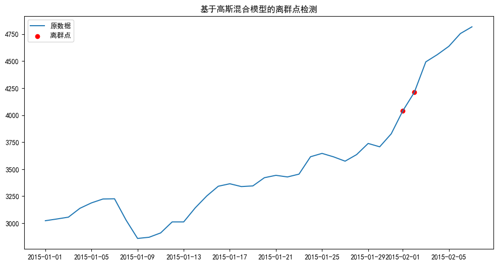
离群点如下:
2015-02-01    4039
2015-02-02    4210
Freq: D, dtype: int32
5.5.1.3 DBSCAN
import numpy as np
import pandas as pd
import matplotlib.pyplot as plt
from sklearn.cluster import DBSCAN
from sklearn.preprocessing import StandardScaler

# 读取数据
data = np.array([
    3023, 3039, 3056, 3138, 3188, 3224, 3226, 3029, 2859, 2870, 2910, 3012, 3012,
    3142, 3252, 3342, 3365, 3339, 3345, 3421, 3443, 3428, 3454, 3615, 3646, 3614, 3574, 3635, 3738,
    3707, 3827, 4039, 4210, 4493, 4560, 4637, 4755, 4817
])

# 将数据转换为时间序列格式
date = pd.date_range(start='2015-01-01', periods=len(data), freq='D')
ts = pd.Series(data, index=date)

# 数据标准化
scaler = StandardScaler()
ts_scaled = scaler.fit_transform(ts.values.reshape(-1, 1))

# 应用DBSCAN进行聚类分析
dbscan = DBSCAN(eps=0.5, min_samples=5)
clusters = dbscan.fit_predict(ts_scaled)

# 获取离群点
outliers = ts[clusters == -1]

# 绘制时序图和离群点
plt.figure(figsize=(12, 6))
plt.plot(ts, label='原数据')
plt.scatter(outliers.index, outliers, color='red', label='离群点')
plt.title('基于DBSCAN的离群点检测')
plt.legend()
plt.show()

# 打印离群点
print("离群点如下:")
print(outliers)

离群点如下:
2015-02-02    4210
Freq: D, dtype: int32
5.5.1.4 KMeans
- 数据标准化处理,使其均值为0,标准差为1。
- 使用K-Means算法进行聚类分析,并将数据分为3个簇。
- 计算每个数据点到其簇中心的距离。
- 定义一个离群点的阈值(例如,距离大于1.5倍标准差的点可以认为是离群点)。
- 识别并打印离群点。
- 使用散点图绘制所有数据点,并标记出离群点。
import numpy as np
import pandas as pd
import matplotlib.pyplot as plt
from sklearn.cluster import KMeans
from sklearn.preprocessing import StandardScaler

# 读取数据
data = np.array([
    3023, 3039, 3056, 3138, 3188, 3224, 3226, 3029, 2859, 2870, 2910, 3012, 3012,
    3142, 3252, 3342, 3365, 3339, 3345, 3421, 3443, 3428, 3454, 3615, 3646, 3614, 3574, 3635, 3738,
    3707, 3827, 4039, 4210, 4493, 4560, 4637, 4755, 4817
])

# 将数据转换为时间序列格式
date = pd.date_range(start='2015-01-01', periods=len(data), freq='D')
ts = pd.Series(data, index=date)

# 数据标准化
scaler = StandardScaler()
ts_scaled = scaler.fit_transform(ts.values.reshape(-1, 1))

# 使用K-Means进行聚类分析
kmeans = KMeans(n_clusters=3, random_state=0).fit(ts_scaled)
clusters = kmeans.predict(ts_scaled)
cluster_centers = kmeans.cluster_centers_

# 计算每个点到其簇中心的距离
distances = np.linalg.norm(ts_scaled - cluster_centers[clusters], axis=1)

# 定义离群点的阈值(如距离大于1.5倍标准差的点)
threshold = np.mean(distances) + 1.5 * np.std(distances)
outliers = ts[distances > threshold]

# 绘制时序图和离群点
plt.figure(figsize=(12, 6))
plt.plot(ts, label='原数据')
plt.scatter(outliers.index, outliers, color='red', label='离群点')
plt.title('基于K-Means的离群点检测')
plt.legend()
plt.show()

# 打印离群点
print("离群点如下:")
print(outliers)

离群点如下:
2015-02-01    4039
2015-02-02    4210
Freq: D, dtype: int32
import numpy as np
from sklearn.datasets import make_blobs
from sklearn.cluster import KMeans
import matplotlib.pyplot as plt

# 生成模拟数据
X, _ = make_blobs(n_samples=300, centers=4, cluster_std=0.60, random_state=0)

# 添加一些离群点
X = np.concatenate((X, np.random.rand(4, 2) * 4), axis=0)

# 执行KMeans聚类
kmeans = KMeans(n_clusters=4)
kmeans.fit(X)

# 计算每个样本到最近聚类中心的距离
distances = kmeans.transform(X) * np.sqrt((kmeans.cluster_centers_ ** 2).sum(axis=1))

# 计算平均距离
avg_distance = np.mean(distances)

# 定义阈值,用于确定离群点
threshold = 2 * avg_distance

# 标记离群点
outliers = distances > threshold

# 绘制数据点和聚类中心
plt.scatter(X[:, 0], X[:, 1], c=outliers, cmap='gray')
centers = kmeans.cluster_centers_
plt.scatter(centers[:, 0], centers[:, 1], c='red', s=200, alpha=0.75)
plt.show()

本文来自博客园,作者:ZhouSpeaks,转载请注明原文链接:https://www.cnblogs.com/zhouwp/p/18217240

 浙公网安备 33010602011771号