澳大利亚天气预测数据分析

一、选题背景

天气预报我们每天都会关注，我们可以根据未来的天气增减衣物、安排出行，每天的气温、风速风向、相对湿度、空气质量等成为关注的焦点。采用公开数据集：澳大利亚多个地点的大约 10 年的每日天气观测数据，对数据集预处理（重复值，缺失值等），借助图形来实现数据可视化，便于更加直观、清晰、有效地展现出来，使得用户可以从不同的维度观察数据，对数据有更深入地理解，在利用机器学习来进一步分析，为获得未来天气信息提供了有效方法。

二、大数据分析设计方案

1.本数据集的数据内容与数据特征分析

字段名称	字段类型	字段说明
Data	浮点型	观察日期
location	浮点型	气象站位置的通用名称
MinTemp	浮点型	以摄氏度为单位的最低温度
Maxtemp	浮点型	以摄氏度为单位的最高温度
Rainfall	浮点型	以毫米为单位记录的当天降雨量
Evaporation	浮点型	所谓A类锅蒸发量(mm)在24小时到早上9点
Sunshine	浮点型	—天中阳光明媚的小时数
WindGustDir	浮点型	24小时至午夜最强阵风方向
WindGustSpeed	浮点型	至午夜24小时内最强阵风的速度(km\/h)
WindDir9am	浮点型	上午9点的风向
WindDir3pm	浮点型	下午3点的风向
WindSpeed9am	浮点型	上午9点前10分钟的平均风速（km\/h)
WindSpeed3pm	浮点型	午3点前10分钟的平均风速(km\/h)
Humidity9am	浮点型	上午9点的湿度〔百分比)
Humidity3am	浮点型	下午3点的湿度〔百分比)
Pressure9am	浮点型	大气压(hpa)在上午9点降至平均海平面
Pressure3pm	浮点型	下午3点大气压力(hpa)降至平均海平面
Cloud9am	浮点型	上午9点被云遮蔽的天空部分。这是用"oktas"来衡量的，它是一个八分之一。它记录了有多少八分之一的天空被云遮住了。0分表示天空完全晴朗，而8分表示完全阴天。
Cloud3pm	浮点型	下午3点被云遮蔽的天空部分(在"oktas"中:八分之一)。有关值的说明，请参阅Cload9am
Temp9am	浮点型	上午9点的温度(摄氏度)
Temp3pm	浮点型	下午3点的温度(摄氏度)
RainToday	浮点型	如果24小时内到上午9点的降水量(mm)超过1mm为1,否则为0
RainTomorrow	浮点型	以毫米为单位的第二天降雨量，用于创建响应变量Rain Tomorrow，一种衡量"风险"的方法。

2、数据分析的课程设计方案概述

采用公开的数据集：

/www.kaggle.com/datasets/jsphyg/weather-dataset-rattle-package

数据清洗：导入公开数据,缺失值处理，补充缺失值，对数值特征进处理

数据可视化：箱型图,pairplot、分组条形图、heatmap（热力图）等来对第二天是否下雨进行预测

机器学习：在训练集和测试集上分布利用训练好的模型进行预测，xgboost预测正确率以及特征重要性等处理采集到的数据

三、数据分析的步骤

导入需要的库

import numpy as np 
import pandas as pd

import matplotlib.pyplot as plt
import seaborn as sns 
%matplotlib inline

1、数据清洗

data = pd.read_csv(r'weatherAUS.csv')#导入数据
data.info()

data.dropna(subset = ['RainTomorrow','RainToday'],inplace=True)
#缺失值处理（24小时降雨和第二天降雨）
data = data.fillna(-1)#缺失数据填充
 data.tail()#默认显示数据最后5行

 

pd.Series(data['RainTomorrow']).value_counts()
#value_counts 直接用来计算series里面相同数据出现的频率
data.describe()#查找给定系列对象的摘要统计信息

 

2、数据可视化分析

 

 category_features
data_plot = data[['Rainfall','Evaporation','Sunshine'] + ['RainTomorrow']]
data_plot

 

plt.figure()
sns.pairplot(data=data_plot,diag_kind="kde",hue= 'RainTomorrow')
plt.show()#在当天降雨量、蒸发量、阳光小时数判断第二天是否下雨

 根据图可知，第二天的降水量与当天降雨量、蒸发量、阳光小时数有关，前一天降水少，第二天降水的的概率偏高，日照小时数少也与第二天是否下雨有关，日照少，第二天降水的概率偏高。

for col in data[numerical_features].columns:
if col != 'RainTomorrow':
sns.boxplot(x='RainTomorrow',y=col,saturation=0.5,palette='pastel',data=data)
plt.title(col)
plt.show()#箱型图

 

有图可知，预测第二天是否下雨，与各个因素之间的联系，蒸发、当天降雨，大气压强直接的表示不是很清楚，当天日照越长，第二天不会下雨概率高反之，被云遮住的面积多，第二天下雨比不下雨要略高。

 

 

 分组条形图：

plt.figure(figsize=(10,10))
plt.subplot(1,2,1)
plt.title('RainTomorrow')
sns.barplot(x = pd.DataFrame(tlog['Location']).sort_index()['Location'], y = pd.DataFrame(tlog['Location']).sort_index().index, color = "Violet")
plt.subplot(1,2,2)
plt.title('Not RainTomorrow')
sns.barplot(x = pd.DataFrame(flog['Location']).sort_index()['Location'], y = pd.DataFrame(flog['Location']).sort_index().index, color = "Lavender")
plt.show()

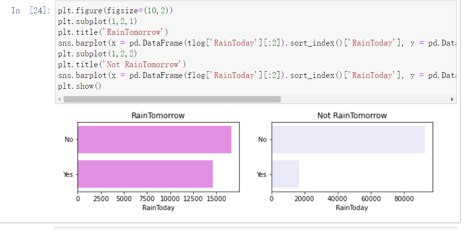
plt.figure(figsize=(10,2))
plt.subplot(1,2,1)
plt.title('RainTomorrow')
sns.barplot(x = pd.DataFrame(tlog['RainToday'][:2]).sort_index()['RainToday'], y = pd.DataFrame(tlog['RainToday'][:2]).sort_index().index, color = "Violet")
plt.subplot(1,2,2)
plt.title('Not RainTomorrow')
sns.barplot(x = pd.DataFrame(flog['RainToday'][:2]).sort_index()['RainToday'], y = pd.DataFrame(flog['RainToday'][:2]).sort_index().index, color = "Lavender")
plt.show()

 3、机器学习

 

## 把所有的相同类别的特征编码为同一个值
def get_mapfunction(x):
mapp = dict(zip(x.unique().tolist(),
range(len(x.unique().tolist()))))
def mapfunction(y):
if y in mapp:
return mapp[y]
else:
return -1
return mapfunction
for i in category_features:
data[i] = data[i].apply(get_mapfunction(data[i]))
data.head()
data.loc[:, 'RainTomorrow'] = data.loc[:, 'RainTomorrow'].map({'No': 0, 'Yes': 1})
from sklearn.model_selection import train_test_split
data_target_part = data['RainTomorrow']
data_features_part = data[[x for x in data.columns if x!='RainTomorrow']]
x_train_val,x_test,y_train_val,y_test = train_test_split(data_features_part,data_target_part,test_size = 0.2, random_state = 42)
x_train,x_val,y_train,y_val = train_test_split(x_train_val,y_train_val,test_size = 0.25, random_state = 42)
## 导入XGBoost模型
from xgboost.sklearn import XGBClassifier
## 定义 XGBoost模型 
clf = XGBClassifier()
# 在训练集上训练XGBoost模型
clf.fit(x_train, y_trai

 

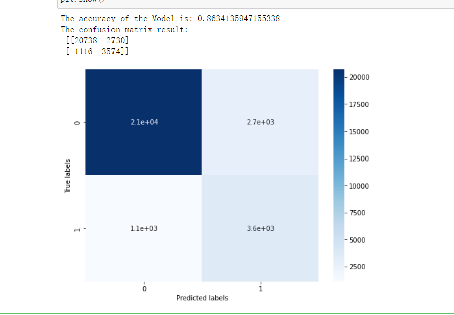
## 在训练集和测试集上分布利用训练好的模型进行预测
train_predict = clf.predict(x_train)
val_predict = clf.predict(x_val)
from sklearn import metrics

print('The accuracy of the Model is:',metrics.accuracy_score(y_val,val_predict))


confusion_matrix_result = metrics.confusion_matrix(val_predict,y_val)
print('The confusion matrix result:\n',confusion_matrix_result)


plt.figure(figsize=(8, 6))
sns.heatmap(confusion_matrix_result, annot=True, cmap='Blues')
plt.xlabel('Predicted labels')
plt.ylabel('True labels')
plt.show()

 

 

 

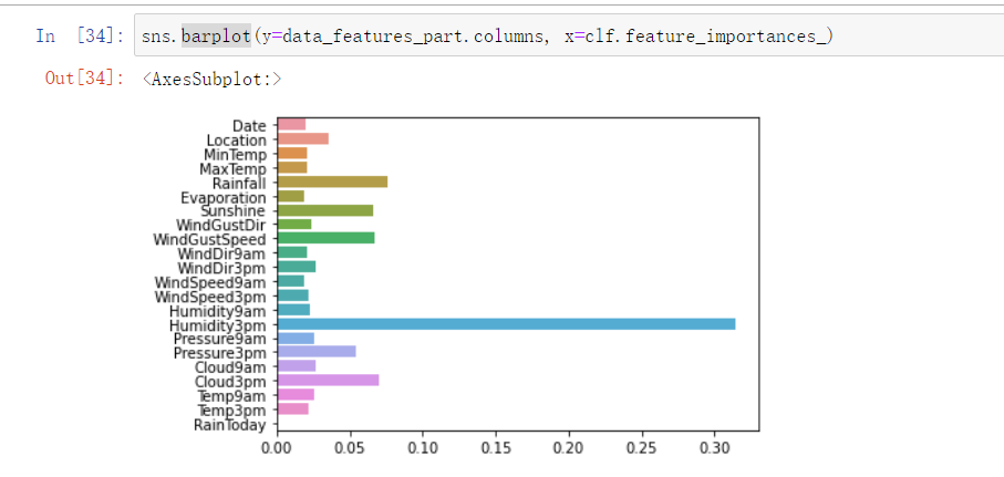
from sklearn.metrics import accuracy_score
from xgboost import plot_importance
#预测正确率以及特征重要性，重要特征值越大，说明该特征越重要
def estimate(model,data):

#sns.barplot(data.columns,model.feature_importances_)
ax1=plot_importance(model,importance_type="gain")
ax1.set_title('gain')
ax2=plot_importance(model, importance_type="weight")
ax2.set_title('weight')
ax3 = plot_importance(model, importance_type="cover")
ax3.set_title('cover')
plt.show()
def classes(data,label,test):
model=XGBClassifier()
model.fit(data,label)
ans=model.predict(test)
estimate(model, data)
return ans

ans=classes(x_train,y_train,x_val)
pre=accuracy_score(y_val, ans)
print('acc=',accuracy_score(y_val,ans))

 

from sklearn.model_selection import GridSearchCV
## 定义参数取值范围
learning_rate = [0.3,0.5,0.7]
subsample = [0.8, 0.9]
colsample_bytree = [0.7,0.8]
max_depth = [7,8,9,10]

parameters = { 'learning_rate': learning_rate,
'subsample': subsample,
'colsample_bytree':colsample_bytree,
'max_depth': max_depth}
model = XGBClassifier(n_estimators = 50)

## 进行网格搜索
clf = GridSearchCV(model, parameters, cv=3, scoring='accuracy',verbose=1,n_jobs=-1)
clf = clf.fit(x_train, y_train)

test_predict = clf.predict(x_test)
print('The accuracy of the Model is:',metrics.accuracy_score(y_test,test_predict))

4、附上完整代码

import numpy as np 
import pandas as pd

import matplotlib.pyplot as plt
import seaborn as sns 
%matplotlib inline

data = pd.read_csv(r'weatherAUS.csv')#导入数据
data.info()

data.shape

data.head()

data.dropna(subset = ['RainTomorrow','RainToday'],inplace=True)
#缺失值处理（24小时降雨和第二天降雨）

data = data.fillna(-1)#缺失数据填充

data.tail()#默认显示数据最后5行

pd.Series(data['RainTomorrow']).value_counts()
#value_counts 直接用来计算series里面相同数据出现的频率

data.describe()#查找给定系列对象的摘要统计信息

numerical_features = [x for x in data.columns if data[x].dtype == float]
category_features = [x for x in data.columns if data[x].dtype != float and x != 'RainTomorrow']

numerical_features#数值特征处理

category_features

data_plot = data[['Rainfall','Evaporation','Sunshine'] + ['RainTomorrow']]

data_plot

plt.figure()
sns.pairplot(data=data_plot,diag_kind="kde",hue= 'RainTomorrow')

plt.show()#在当天降雨量、蒸发量、阳光小时数判断第二天是否下雨

for col in data[numerical_features].columns:
if col != 'RainTomorrow':
sns.boxplot(x='RainTomorrow',y=col,saturation=0.5,palette='pastel',data=data)
plt.title(col)
plt.show()#箱型图

tlog={}
for i in category_features:
tlog[i] = data[data['RainTomorrow'] == 'Yes'][i].value_counts()
flog={}
for i in category_features:
flog[i] = data[data['RainTomorrow'] == 'No'][i].value_counts()

tlog

plt.figure(figsize=(10,10))
plt.subplot(1,2,1)
plt.title('RainTomorrow')
sns.barplot(x = pd.DataFrame(tlog['Location']).sort_index()['Location'], y = pd.DataFrame(tlog['Location']).sort_index().index, color = "Violet")
plt.subplot(1,2,2)
plt.title('Not RainTomorrow')
sns.barplot(x = pd.DataFrame(flog['Location']).sort_index()['Location'], y = pd.DataFrame(flog['Location']).sort_index().index, color = "Lavender")
plt.show()

plt.figure(figsize=(10,2))
plt.subplot(1,2,1)
plt.title('RainTomorrow')
sns.barplot(x = pd.DataFrame(tlog['RainToday'][:2]).sort_index()['RainToday'], y = pd.DataFrame(tlog['RainToday'][:2]).sort_index().index, color = "Violet")
plt.subplot(1,2,2)
plt.title('Not RainTomorrow')
sns.barplot(x = pd.DataFrame(flog['RainToday'][:2]).sort_index()['RainToday'], y = pd.DataFrame(flog['RainToday'][:2]).sort_index().index, color = "Lavender")
plt.show()

## 把所有的相同类别的特征编码为同一个值
def get_mapfunction(x):
mapp = dict(zip(x.unique().tolist(),
range(len(x.unique().tolist()))))
def mapfunction(y):
if y in mapp:
return mapp[y]
else:
return -1
return mapfunction

for i in category_features:
data[i] = data[i].apply(get_mapfunction(data[i]))

data.head()

data.loc[:, 'RainTomorrow'] = data.loc[:, 'RainTomorrow'].map({'No': 0, 'Yes': 1})

from sklearn.model_selection import train_test_split

data_target_part = data['RainTomorrow']
data_features_part = data[[x for x in data.columns if x!='RainTomorrow']]

x_train_val,x_test,y_train_val,y_test = train_test_split(data_features_part,data_target_part,test_size = 0.2, random_state = 42)
x_train,x_val,y_train,y_val = train_test_split(x_train_val,y_train_val,test_size = 0.25, random_state = 42)

## 导入XGBoost模型
from xgboost.sklearn import XGBClassifier
## 定义 XGBoost模型 
clf = XGBClassifier()
# 在训练集上训练XGBoost模型
clf.fit(x_train, y_train)

## 在训练集和测试集上分布利用训练好的模型进行预测
train_predict = clf.predict(x_train)
val_predict = clf.predict(x_val)
from sklearn import metrics

print('The accuracy of the Model is:',metrics.accuracy_score(y_val,val_predict))

confusion_matrix_result = metrics.confusion_matrix(val_predict,y_val)
print('The confusion matrix result:\n',confusion_matrix_result)

plt.figure(figsize=(8, 6))
sns.heatmap(confusion_matrix_result, annot=True, cmap='Blues')
plt.xlabel('Predicted labels')
plt.ylabel('True labels')
plt.show()

sns.barplot(y=data_features_part.columns, x=clf.feature_importances_)

from sklearn.metrics import accuracy_score
from xgboost import plot_importance
#预测正确率以及特征重要性，重要特征值越大，说明该特征越重要
def estimate(model,data):

#sns.barplot(data.columns,model.feature_importances_)
ax1=plot_importance(model,importance_type="gain")
ax1.set_title('gain')
ax2=plot_importance(model, importance_type="weight")
ax2.set_title('weight')
ax3 = plot_importance(model, importance_type="cover")
ax3.set_title('cover')
plt.show()
def classes(data,label,test):
model=XGBClassifier()
model.fit(data,label)
ans=model.predict(test)
estimate(model, data)
return ans
ans=classes(x_train,y_train,x_val)
pre=accuracy_score(y_val, ans)
print('acc=',accuracy_score(y_val,ans))

## 从sklearn库中导入网格调参函数
from sklearn.model_selection import GridSearchCV

## 定义参数取值范围
learning_rate = [0.3,0.5,0.7]
subsample = [0.8, 0.9]
colsample_bytree = [0.7,0.8]
max_depth = [7,8,9,10]

parameters = { 'learning_rate': learning_rate,
'subsample': subsample,
'colsample_bytree':colsample_bytree,
'max_depth': max_depth}
model = XGBClassifier(n_estimators = 50)

## 进行网格搜索
clf = GridSearchCV(model, parameters, cv=3, scoring='accuracy',verbose=1,n_jobs=-1)
clf = clf.fit(x_train, y_train)

best_params = clf.best_params_

bp = list(best_params.values())


clf = XGBClassifier(colsample_bytree = bp[0], learning_rate = bp[1], max_depth= bp[2], subsample = bp[3])
# 在训练集上训练XGBoost模型
clf.fit(x_train, y_train)

train_predict = clf.predict(x_train)
val_predict = clf.predict(x_val)

print('The accuracy of the Model is:',metrics.accuracy_score(y_val,val_predict))

confusion_matrix_result = metrics.confusion_matrix(val_predict,y_val)
print('The confusion matrix result:\n',confusion_matrix_result)

plt.figure(figsize=(8, 6))
sns.heatmap(confusion_matrix_result, annot=True, cmap='Blues')
plt.xlabel('Predicted labels')
plt.ylabel('True labels')
plt.show()

test_predict = clf.predict(x_test)
print('The accuracy of the Model is:',metrics.accuracy_score(y_test,test_predict))

 

 四、总结

1.首先根据温湿度数据进行的分析，温度从早上低到中午高再到晚上低，湿度和温度的趋势相反，通过相关系数发现温度和湿度有强烈的负相关关系，经查阅资料发现因为随着温度升高水蒸汽蒸发加剧，空气中水分降低湿度降低。当然，湿度同时受气压和雨水的影响，下雨湿度会明显增高。
2.经查阅资料空气质量不仅跟工厂、汽车等排放的烟气、废气等有关，更为重要的是与气象因素有关。由于昼夜温差明显变化，当地面温度高于高空温度时，空气上升，污染物易被带到高空扩散；当地面温度低于一定高度的温度时，天空形成逆温层，它像一个大盖子一样压在地面上空，使地表空气中各种污染物不易扩散。一般在晚间和清晨影响较大，而当太阳出来后，地面迅速升温，逆温层就会逐渐消散，于是污染空气也就扩散了。
3.第二天是否会下雨，与之相光的因素有很多，对于天气进行预测，可以让我们对第二天的天气有一个大致的判断，也给我们日常生活和出行带来了极大的便利，防患于未然。
结论：

数据的挖掘和分析对于我们平常的生活过程中带来了许多的便利，带面对大量数据是，可以清晰直观的了解数据说明的的内容，数据分析和机器学习，节省了大量的人力。本次实验对于预期目标的基本实现。

收获：

本次学习对于python的应用，大数据分析和机器学习的知识点有了更加深入的学习，对于不熟悉的地方逐渐掌握，但是整体而言，对于数据分析和机器学习本人还是比较生疏，整体衔接不顺畅，在以后的学习中继续查漏补缺。2022-12-17