感知机的理解和实现

感知机

感知机是根据输入实例的特征向量 x 对其进行二类分类的线性模型：
f(x)=sign(w⋅x+b)

感知机模型对应于输入空间（特征空间）中的分离超平面 w⋅x+b=0。其中w是超平面的法向量，b是超平面的截距。
可见感知机是一种线性分类模型，属于判别模型。

感知机学习的假设

感知机学习的重要前提假设是训练数据集是线性可分的。

感知机学习策略

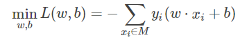
感知机学的策略是极小化损失函数。

损失函数的一个自然选择是误分类点的总数。但是，这样的损失函数不是参数 w, b的连续可导的函数，不易于优化。所以通常是选择误分类点到超平面 S 的总距离：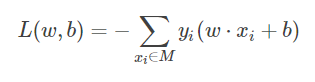

学习的策略就是求得使 L(w,b) 为最小值的 w 和 b。其中 M 是误分类点的集合。

---

 感知机学习的算法

感知机学习算法是基于随机梯度下降法的对损失函数的最优化算法，有原始形式和对偶形式，算法简单易于实现。

原始形式

首先，任意选取一个超平面 w0,b0，然后用梯度下降法不断地极小化目标函数。极小化的过程中不是一次使 M 中所有误分类点得梯度下降，而是一次随机选取一个误分类点，使其梯度下降。

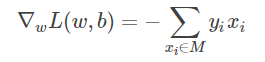
随机选取一个误分类点(xi,yi)，对 w,b 进行更新：
w←w+ηyixi

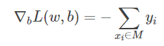
b←b+ηyi

其中 η(0<η≤1)是学习率。

对偶形式

对偶形式的基本想法是，将 w 和 b 表示为是咧 xi和标记 yi的线性组合的形式，通过求解其系数而得到 w 和 b。
w←w+ηyixi

b←b+ηyi

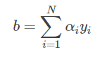
逐步修改 w,b，设修改 n 次，则 w,b 关于 (xi,yi) 的增量分别是 αiyixi和 αiyi, 这里 αi=niη。最后学习到的 w,b 可以分别表示为：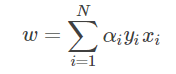

这里， αi≥0, i=1,2,...,N ，当 η=1时，表示第i个是实例点由于误分类而进行更新的次数，实例点更新次数越多，说明它距离分离超平面越近，也就越难区分，该点对学习结果的影响最大。
感知机模型对偶形式：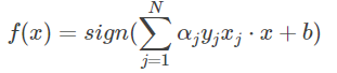

其中
α=(α1,α2,...,αN)T

学习时初始化 α←0,b←0α←0,b←0, 在训练集中找分类错误的点，即：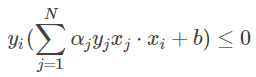

然后更新：
αi←αi+η     这里为什么这样更新，请看推导文章感知机对偶形式 梯度下降法的推导过程

b←b+ηyi

知道训练集中所有点正确分类
对偶形式中训练实例仅以内积的形式出现，为了方便，可以预先将训练集中实例间的内积计算出来以矩阵的形式存储，即 Gram 矩阵。

---

 总结

• 当训练数据集线性可分的时候，感知机学习算法是收敛的，感知机算法在训练数据集上的误分类次数 k 满足不等式:

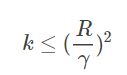
具体证明可见 李航《统计学习方法》或 林轩田《机器学习基石》。
当训练当训练数据集线性可分的时候，感知机学习算法存在无穷多个解，其解由于不同的初值或不同的迭代顺序而可能不同，即存在多个分离超平面能把数据集分开。

感知机学习算法简单易求解，但一般的感知机算法不能解决异或等线性不可分的问题。

感知机（采用原始形式）

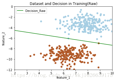
创建感知机模型的原始形式的类，并在训练集上训练，测试集上简单测试。

class PerceptronRaw():
    def __init__(self):
        self.W = None;
        self.bias = None;

    def fit(self, x_train, y_train, learning_rate=0.05, n_iters=100, plot_train=True):
        print("开始训练...")
        num_samples, num_features = x_train.shape
        self.W = np.random.randn(num_features)
        self.bias = 0

        while True:
            erros_examples = []
            erros_examples_y = [] 
            # 查找错误分类的样本点
            for idx in range(num_samples):
                example = x_train[idx]
                y_idx = y_train[idx]
                # 计算距离
                distance = y_idx * (np.dot(example, self.W) + self.bias)
                if distance <= 0:
                    erros_examples.append(example)
                    erros_examples_y.append(y_idx)
            if len(erros_examples) == 0:
                break;
            else:
                # 随机选择一个错误分类点，修正参数
                random_idx = np.random.randint(0, len(erros_examples))
                choosed_example = erros_examples[random_idx]
                choosed_example_y = erros_examples_y[random_idx]
                self.W = self.W + learning_rate * choosed_example_y * choosed_example
                self.bias = self.bias + learning_rate * choosed_example_y    
        print("训练结束")

        # 绘制训练结果部分
        if plot_train is True:
            x_hyperplane = np.linspace(2, 10, 8)
            slope = -self.W[0]/self.W[1]
            intercept = -self.bias/self.W[1]
            y_hpyerplane = slope * x_hyperplane + intercept

            plt.xlabel("feature_1")
            plt.ylabel("feature_2")
            plt.xlim((2, 10))
            plt.ylim((-12, 0))
            plt.title("Dataset and Decision in Training(Raw)")
            plt.scatter(x_train[:, 0], x_train[:, 1], c=y_train, s=30, cmap=plt.cm.Paired)
            plt.plot(x_hyperplane, y_hpyerplane, color='g', label='Decision_Raw')
            plt.legend(loc='upper left')
            plt.show()

    def predict(self, x):
        if self.W is None or self.bias is None:
            raise NameError("模型未训练")
        y_predict = np.sign(np.dot(x, self.W) + self.bias)
        return y_predict

感知机（采用对偶形式）

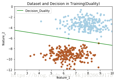
创建感知机模型的对偶形式的类，并在训练集上训练，测试集上简单测试。

class PerceptronDuality():
    def __init__(self):
        self.alpha = None
        self.bias = None
        self.W = None
    def fit(self, x_train, y_train, learning_rate=1, n_iters=100, plot_train=True):
        print("开始训练...")
        num_samples, num_features = x_train.shape
        self.alpha = np.zeros((num_samples,))
        self.bias = 0

        # 计算 Gram 矩阵
        gram = np.dot(x_train, x_train.T)

        while True:
            error_count = 0
            for idx in range(num_samples):
                inner_product = gram[idx]
                y_idx = y_train[idx]
                distance = y_idx * (np.sum(self.alpha * y_train * inner_product) + self.bias)
                # 如果有分类错误点，修正 alpha 和 bias，跳出本层循环，重新遍历数据计算，开始新的循环
                if distance <= 0:
                    error_count += 1
                    self.alpha[idx] = self.alpha[idx] + learning_rate
                    self.bias = self.bias + learning_rate * y_idx
                    break  
            # 数据没有错分类点，跳出 while 循环
            if error_count == 0:
                break
        self.W = np.sum(self.alpha * y_train * x_train.T, axis=1)       
        print("训练结束")

        # 绘制训练结果部分
        if plot_train is True:
            x_hyperplane = np.linspace(2, 10, 8)           
            slope = -self.W[0]/self.W[1]
            intercept = -self.bias/self.W[1]
            y_hpyerplane = slope * x_hyperplane + intercept

            plt.xlabel("feature_1")
            plt.ylabel("feature_2")
            plt.xlim((2, 10))
            plt.ylim((-12, 0))
            plt.title("Dataset and Decision in Training(Duality)")
            plt.scatter(x_train[:, 0], x_train[:, 1], c=y_train, s=30, cmap=plt.cm.Paired)
            plt.plot(x_hyperplane, y_hpyerplane, color='g', label='Decision_Duality')
            plt.legend(loc='upper left')
            plt.show()

    def predict(self, x):
        if self.alpha is None or self.bias is None:
            raise NameError("模型未训练")
        y_predicted = np.sign(np.dot(x, self.W) + self.bias)
        return y_predicted

---

 详细代码链接：

https://github.com/kenjewu/Machine_Learning_ALS/blob/master/perceptron.ipynb
如果该代码对您的工作学习有帮助，请点个star。欢迎大家指正，提出更好的写法意见，转载请贴上引用。

---

 引用

《统计学习方法》 李航
《机器学习基石》 林轩田

---

 参考：https://blog.csdn.net/wkj1026639175/article/details/79827923

https://blog.csdn.net/mishifangxiangdefeng/article/details/104641962/?utm_medium=distribute.pc_relevant.none-task-blog-baidujs_baidulandingword-0&spm=1001.2101.3001.4242