如何使用 pytorch 实现 yolov3
前言
看了 Yolov3 的论文之后,发现这论文写的真的是很简短,神经网络的具体结构和损失函数的公式都没有给出。所以这里参考了许多前人的博客和代码,下面进入正题。
网络结构
Yolov3 将主干网络换成了 darknet53,整体的网络结构如下图所示(图片来自【论文解读】Yolo三部曲解读——Yolov3):
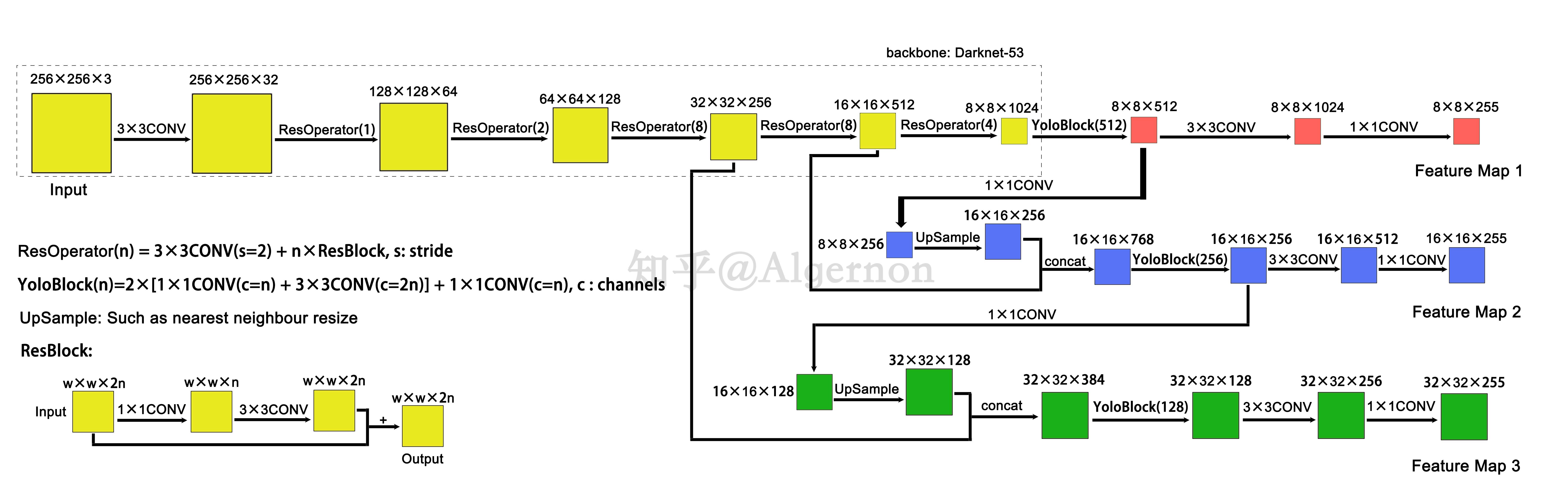
这里的 CONV 具体结构是 1 个 Conv2d + 1 个 BatchNorm2d + 1个 LeakyReLU (除了 Feature Map 1、2、3 前的 1×1 CONV),代码如下:
class ConvBlock(nn.Module):
    """ 卷积块 """

    def __init__(self, in_channels, out_channels, kernel_size=3, stride=1, padding=1):
        super().__init__()
        self.features = nn.Sequential(
            nn.Conv2d(in_channels, out_channels, kernel_size,
                      stride, padding, bias=False),
            nn.BatchNorm2d(out_channels),
            nn.LeakyReLU(0.1)
        )

    def forward(self, x):
        return self.features(x)
ResBlock 里面进行了两次卷积,最后还有一个跳连接,代码如下:
class ResidualUnit(nn.Module):
    """ 残差单元 """

    def __init__(self, in_channels: int):
        super().__init__()
        self.features = nn.Sequential(
            ConvBlock(in_channels, in_channels//2, 1, padding=0),
            ConvBlock(in_channels//2, in_channels, 3),
        )

    def forward(self, x):
        y = self.features(x)
        return x+y
ResOperator(n) 包括一个卷积核大小为 3×3、步长为 2 的 Convolutional 和 n 个 ResBlock,代码如下:
class ResidualBlock(nn.Module):
    """ 残差块 """

    def __init__(self, in_channels: int, n_residuals=1):
        """
        Parameters
        ----------
        in_channels: int
            输入通道数

        n_residuals: int
            残差单元的个数
        """
        super().__init__()
        self.conv = ConvBlock(in_channels, in_channels*2, 3, stride=2)
        self.residual_units = nn.Sequential(*[
            ResidualUnit(2*in_channels) for _ in range(n_residuals)
        ])

    def forward(self, x):
        return self.residual_units(self.conv(x))
在 Darknet53 中共有 1+2+8+8+4=23 个 ResOperator,假设输入 Darknet53 的图像维度为 256×256×3,那么最后会输出 3 个特征图,维度分别是 32×32×256、16×16×512 和 8×8×1024,大小分别是原始图像的 1/8、1/16 和 1/32(说明输入 Darknet 的图像的宽高需要是 32 的倍数),这些特征图会在后面接着进行卷积。
class Darknet(nn.Module):
    """ 主干网络 """

    def __init__(self):
        super().__init__()
        self.conv = ConvBlock(3, 32, 3)
        self.residuals = nn.ModuleList([
            ResidualBlock(32, 1),
            ResidualBlock(64, 2),
            ResidualBlock(128, 8),
            ResidualBlock(256, 8),
            ResidualBlock(512, 4),
        ])

    def forward(self, x):
        """
        Parameters
        ----------
        x: Tensor of shape `(N, 3, H, W)`
            输入图像

        Returns
        -------
        x1: Tensor of shape `(N, 1024, H/32, W/32)`
        x2: Tensor of shape `(N, 512, H/16, W/16)`
        x3: Tensor of shape `(N, 256, H/8, W/8)`
        """
        x3 = self.conv(x)
        for layer in self.residuals[:-2]:
            x3 = layer(x3)

        x2 = self.residuals[-2](x3)
        x1 = self.residuals[-1](x2)
        return x1, x2, x3
8×8×1024 特征图会先经过 YoloBlock,得到 8×8×512 的特征图 x1,YoloBlock 的代码如下所示:
class YoloBlock(nn.Module):
    """ Yolo 块 """

    def __init__(self, in_channels: int, out_channels: int):
        super().__init__()
        self.features = nn.Sequential(*[
            ConvBlock(in_channels, out_channels, 1, padding=0),
            ConvBlock(out_channels, out_channels*2, 3, padding=1),
            ConvBlock(out_channels*2, out_channels, 1, padding=0),
            ConvBlock(out_channels, out_channels*2, 3, padding=1),
            ConvBlock(out_channels*2, out_channels, 1, padding=0),
        ])

    def forward(self, x):
        return self.features(x)
x1 在经过后续的两次卷积后,得到维度为 8×8×255 的第一个特征图 y1,后面会解释特征图的含义。
为了融合 x1 中所包含的高级语义, Yolov3 先 x1 进行了 1×1 大小的卷积,减少通道数,接着进行上采样,使特征图的维度变为 16×16×256,再与 darknet53 输出的 16×16×512 的特征图沿着通道方向进行连结,得到 16×16×768 的特征图。该特征图经过 YoloBlock 和后续两次卷积后得到维度为 16×16×255 的第二个特征图 y2。y3 同理。总结下来整个 Yolov3 的代码为:
class Yolo(nn.Module):
    """ Yolo 神经网络 """

    def __init__(self, n_classes: int, image_size=416, anchors: list = None, nms_thresh=0.45):
        """
        Parameters
        ----------
        n_classes: int
            类别数

        image_size: int
            图片尺寸,必须是 32 的倍数

        anchors: list
            输入图像大小为 416 时对应的先验框

        nms_thresh: float
            非极大值抑制的交并比阈值,值越大保留的预测框越多
        """
        super().__init__()
        if image_size <= 0 or image_size % 32 != 0:
            raise ValueError("image_size 必须是 32 的倍数")

        # 先验框
        anchors = anchors or [
            [[116, 90], [156, 198], [373, 326]],
            [[30, 61], [62, 45], [59, 119]],
            [[10, 13], [16, 30], [33, 23]]
        ]
        anchors = np.array(anchors, dtype=np.float32)
        anchors = anchors*image_size/416
        self.anchors = anchors.tolist()

        self.n_classes = n_classes
        self.image_size = image_size

        self.darknet = Darknet()
        self.yolo1 = YoloBlock(1024, 512)
        self.yolo2 = YoloBlock(768, 256)
        self.yolo3 = YoloBlock(384, 128)
        # YoloBlock 后面的卷积部分
        out_channels = (n_classes+5)*3
        self.conv1 = nn.Sequential(*[
            ConvBlock(512, 1024, 3),
            nn.Conv2d(1024, out_channels, 1)
        ])
        self.conv2 = nn.Sequential(*[
            ConvBlock(256, 512, 3),
            nn.Conv2d(512, out_channels, 1)
        ])
        self.conv3 = nn.Sequential(*[
            ConvBlock(128, 256, 3),
            nn.Conv2d(256, out_channels, 1)
        ])
        # 上采样
        self.upsample1 = nn.Sequential(*[
            nn.Conv2d(512, 256, 1),
            nn.Upsample(scale_factor=2)
        ])
        self.upsample2 = nn.Sequential(*[
            nn.Conv2d(256, 128, 1),
            nn.Upsample(scale_factor=2)
        ])

        # 探测器,用于处理输出的特征图,后面会讲到
        self.detector = Detector(
            self.anchors, image_size, n_classes, conf_thresh=0.1, nms_thresh=nms_thresh)

    def forward(self, x):
        """
        Parameters
        ----------
        x: Tensor of shape `(N, 3, H, W)`
            输入图像

        Returns
        -------
        y1: Tensor of shape `(N, 255, H/32, W/32)`
            最小的特征图

        y2: Tensor of shape `(N, 255, H/16, W/16)`
            中等特征图

        y3: Tensor of shape `(N, 255, H/8, W/8)`
            最大的特征图
        """
        x1, x2, x3 = self.darknet(x)
        x1 = self.yolo1(x1)
        y1 = self.conv1(x1)

        x2 = self.yolo2(torch.cat([self.upsample1(x1), x2], 1))
        y2 = self.conv2(x2)

        x3 = self.yolo3(torch.cat([self.upsample2(x2), x3], 1))
        y3 = self.conv3(x3)

        return y1, y2, y3
先验框
k-means 算法
在介绍先验框之前,有必要说下 k-means 聚类算法。假设我们有一个样本集 \(D=\left\{ \boldsymbol{x_1}, \boldsymbol{x_2}, ..., \boldsymbol{x_m} \right\}\) 包含 \(m\) 个样本,其中每一个样本 \(\boldsymbol{x_i}=[x_{i1}, x_{i2}, ..., x_{in}]^T\) 是 \(n\) 维空间中的一个点。k-means 算法会将样本集划分为 \(k\) 个不相交的簇 \(\left\{ C_l | l=1,2,...,k \right\}\) 来最小化平方误差:
其中 $\boldsymbol{\mu_j}=\frac{1}{|C_j|}\sum_{\boldsymbol{x}\in C_j} \boldsymbol{x} $ 是簇 \(C_j\) 的均值向量(聚类中心)。简单来说,上面这个公式刻画了簇内样本围绕簇均值向量的紧密程度,\(E\) 值越小则簇内样本相似度越高。k-means 算法法采用了贪心策略,通过迭代优化来近似求解 \(\boldsymbol{\mu_j}\)。流程如下:
- 从样本集 \(D\) 中随机选择 \(k\) 个样本作为初始均值向量 \(\left\{ \boldsymbol{\mu_1},\boldsymbol{\mu_2},...,\boldsymbol{\mu_k} \right\}\)
- 对于每一个样本 \(\boldsymbol{x_i} (1\le i \le m)\) 计算它与各聚类中心 $\boldsymbol{\mu_j}\left(1\le j \le k \right) $的距离 \(d_{ij}=|| \boldsymbol{x_i} - \boldsymbol{\mu_j} ||_2\)
- 根据距离最近的均值向量确定的簇标记 \(\lambda_{i}={\rm argmin} _{j \in \left\{ 1,2,...,k \right\} d_{ij} }\),将 \(\boldsymbol{x_i}\) 划入响应的簇 \(C_{\lambda_i}=C_{\lambda_{i} } \cup \{ \boldsymbol{x_i} \}\)
- 重新计算聚类中心 $\boldsymbol{\mu_j'}=\frac{1}{|C_j|}\sum_{\boldsymbol{x}\in C_j} \boldsymbol{x} $
- 如果所有的聚类中心都满足 \(\boldsymbol{\mu_j'}=\boldsymbol{\mu_j}(1\le j \le k)\),聚类结束,否则回到步骤 2 接着迭代
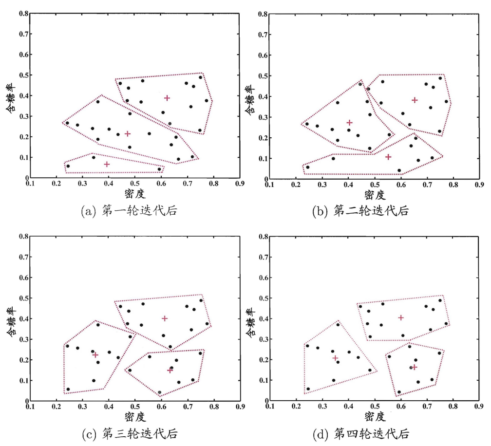
下图展示了在西瓜的含糖量和密度张成的二维空间中, \(k=3\) 时 k-means 算法迭代过程(图片来自周志强老师的《机器学习》)
Yolov3 中的 k-means
上述的 k-means 算法使用欧式距离作为样本和聚类中心的距离度量,而 Yolov3 中则换了一种距离度量方式。假设边界框样本集为 \(D=\left\{ \boldsymbol{x_1}, \boldsymbol{x_2}, ..., \boldsymbol{x_m} \right\}\) 包含 \(m\) 个边界框,其中每一个样本 \(\boldsymbol{x_i}=[x_{i1}, x_{i2}, x_{i3}, x_{i4}]^T=[0, 0, w, h]^T\) 是 \(4\) 维空间中的一个点(已归一化),这里把所有的边界框的左上角都平移到了原点处。在 Yolov3 中,样本 \(\boldsymbol{x_i}\) 和聚类中心 \(\boldsymbol{\mu_j}\) 的距离写作
可以看到样本和聚类中心的交并比越大,距离就越小,将这个公式作为距离度量可以说是十分的巧妙。
Yolov3 的作者对 COCO 数据集中的边界框进行了 k-means 聚类,得到了 9 个先验框,这些先验框是归一化后的先验框再乘以图像尺寸 416 得到的,由于神经网络输出了 3 个不同大小的特征图,所以将先验框分为 3 类:
- 大尺度先验框:[116, 90], [156, 198], [373, 326],对应最小的那个特征图 13×13×255
- 中尺度先验框:[30, 61], [62, 45], [59, 119],对应中等大小的特征图 26×26×255
- 小尺度先验框:[10, 13], [16, 30], [33, 23],对应最大的特征图 52×52×255
在训练自己的数据集时,COCO数据集的先验框可能不适用,所以应该对边界框重新聚类。下面给出聚类的代码:
# coding:utf-8
import glob
from xml.etree import ElementTree as ET

import numpy as np


def iou(box: np.ndarray, boxes: np.ndarray):
    """ 计算一个边界框和多个边界框的交并比

    Parameters
    ----------
    box: `~np.ndarray` of shape `(4, )`
        边界框

    boxes: `~np.ndarray` of shape `(n, 4)`
        其他边界框

    Returns
    -------
    iou: `~np.ndarray` of shape `(n, )`
        交并比
    """
    # 计算交集
    xy_max = np.minimum(boxes[:, 2:], box[2:])
    xy_min = np.maximum(boxes[:, :2], box[:2])
    inter = np.clip(xy_max-xy_min, a_min=0, a_max=np.inf)
    inter = inter[:, 0]*inter[:, 1]

    # 计算并集
    area_boxes = (boxes[:, 2]-boxes[:, 0])*(boxes[:, 3]-boxes[:, 1])
    area_box = (box[2]-box[0])*(box[3]-box[1])

    retun inter/(area_box+area_boxes-inter)


class AnchorKmeans:
    """ 先验框聚类 """

    def __init__(self, annotation_dir: str):
        self.annotation_dir = annotation_dir
        self.bbox = self.get_bbox()

    def get_bbox(self) -> np.ndarray:
        """ 获取所有的边界框 """
        bbox = []

        for path in glob.glob(f'{self.annotation_dir}/*xml'):
            root = ET.parse(path).getroot()

            # 图像的宽度和高度
            w = int(root.find('size/width').text)
            h = int(root.find('size/height').text)

            # 获取所有边界框
            for obj in root.iter('object'):
                box = obj.find('bndbox')

                # 归一化坐标
                xmin = int(box.find('xmin').text)/w
                ymin = int(box.find('ymin').text)/h
                xmax = int(box.find('xmax').text)/w
                ymax = int(box.find('ymax').text)/h

                bbox.append([0, 0, xmax-xmin, ymax-ymin])

        return np.array(bbox)

    def get_cluster(self, n_clusters=9, metric=np.median):
        """ 获取聚类结果

        Parameters
        ----------
        n_clusters: int
            聚类数

        metric: callable
            选取聚类中心点的方式
        """
        rows = self.bbox.shape[0]

        if rows < n_clusters:
            raise ValueError("n_clusters 不能大于边界框样本数")

        last_clusters = np.zeros(rows)
        clusters = np.ones((n_clusters, 2))
        distances = np.zeros((rows, n_clusters))  # type:np.ndarray

        # 随机选取出几个点作为聚类中心
        # np.random.seed(1)
        clusters = self.bbox[np.random.choice(rows, n_clusters, replace=False)]

        # 开始聚类
        while True:
            # 计算距离
            distances = 1-self.iou(clusters)

            # 将每一个边界框划到一个聚类中
            nearest_clusters = distances.argmin(axis=1)

            # 如果聚类中心不再变化就退出
            if np.array_equal(nearest_clusters, last_clusters):
                break

            # 重新选取聚类中心
            for i in range(n_clusters):
                clusters[i] = metric(self.bbox[nearest_clusters == i], axis=0)

            last_clusters = nearest_clusters

        return clusters[:, 2:]

    def average_iou(self, clusters: np.ndarray):
        """ 计算 IOU 均值

        Parameters
        ----------
        clusters: `~np.ndarray` of shape `(n_clusters, 2)`
            聚类中心
        """
        clusters = np.hstack((np.zeros((clusters.shape[0], 2)), clusters))
        return np.mean([np.max(iou(bbox, clusters)) for bbox in self.bbox])

    def iou(self, clusters: np.ndarray):
        """ 计算所有边界框和所有聚类中心的交并比

        Parameters
        ----------
        clusters: `~np.ndarray` of shape `(n_clusters, 4)`
            聚类中心

        Returns
        -------
        iou: `~np.ndarray` of shape `(n_bbox, n_clusters)`
            交并比
        """
        bbox = self.bbox
        A = self.bbox.shape[0]
        B = clusters.shape[0]

        xy_max = np.minimum(bbox[:, np.newaxis, 2:].repeat(B, axis=1),
                            np.broadcast_to(clusters[:, 2:], (A, B, 2)))
        xy_min = np.maximum(bbox[:, np.newaxis, :2].repeat(B, axis=1),
                            np.broadcast_to(clusters[:, :2], (A, B, 2)))

        # 计算交集面积
        inter = np.clip(xy_max-xy_min, a_min=0, a_max=np.inf)
        inter = inter[:, :, 0]*inter[:, :, 1]

        # 计算每个矩阵的面积
        area_bbox = ((bbox[:, 2]-bbox[:, 0])*(bbox[:, 3] -
                     bbox[:, 1]))[:, np.newaxis].repeat(B, axis=1)
        area_clusters = ((clusters[:, 2] - clusters[:, 0])*(
            clusters[:, 3] - clusters[:, 1]))[np.newaxis, :].repeat(A, axis=0)

        return inter/(area_bbox+area_clusters-inter)
来计算一下 VOC2007 数据集的聚类结果,由于聚类结果会受到初始点的影响,所以每次运行的结果会不一样,但是平均 IOU 应该是相近的:
root = 'data/VOCtrainval_06-Nov-2007/VOCdevkit/VOC2007/Annotations'
model = AnchorKmeans(root)

t0 = time()
clusters = model.get_cluster(9)
t1 = time()

print(f'耗时: {t1-t0} s')
print('聚类结果:\n', clusters*416)
print('平均 IOU:', model.average_iou(clusters))
特征图分析
对于每个特征图,我们给他分配了 3 个先验框,如果数据集中有 C 个类,那么在特征图的每个像素点处,我们会得到 3 个预测框,每个预测框预测一个 (4+1+C) 维的向量。假设我们使用 COCO 数据集,并将输入神经网络的图片缩放为 416×416 的大小。由于我们的 COCO 数据集有 80 个类,所以在最小的特征图的维度就应该是 13×13×(4+1+80)*3 即 13×13×255,为了方便理解和索引,我们将这个特征图的维度 reshape 为 13×13×3×85。将 reshape 后的特征图记为 y,那么 y[i, j, k] 的结果就会如下图所示:
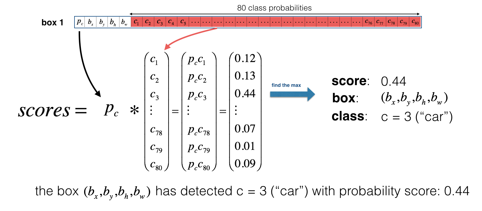
我们取到了一个 85 维的向量,上图中这个向量的第1个元素 \(p_c\) 是 objectness score,代表这个预测框对包含物体的自信程度,我们将它重新记作 \(P(obj)\)。第 2 到 5 个元素 \((b_x, b_y, b_h, b_w)\) 表示这个预测框的中心点位置和宽高。后面 80 个元素 class probabilities 代表了在预测框含有物体的条件下,先验框中是某个类别 \(c_i\) 的概率,所以这里的类别概率是一个条件概率 \(P(c_i|obj)\),在我们使用 Yolov3 进行推理的时候,预测框上标注的概率是先验概率,也就是 \(P(c_i)=P(obj)*P(c_i|obj)\),对应到上图就是那个 score(也用来 nms)。实际在代码中我们会把边界框的位置和宽高放到前 4 个元素,objectness score 放到第 5 个元素,后面的就是 class probabilities。
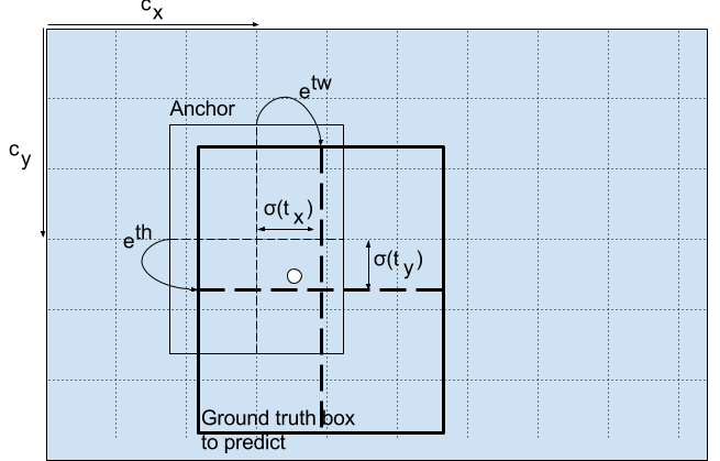
实际上我们不会直接预测 \((b_x, b_y, b_h, b_w)\),而是预测偏差量 \((t_x,t_y,t_w,t_h)\) ,也就是说上图中的第 2 到 5 个元素应该替换为偏差量。至于为什么要换成偏差量,原因应该是\((b_x, b_y, b_h, b_w)\) 的数值大小和 objectness score 以及 class probilities 差太多了,会给训练带来困难。这里先给出 \((t_x,t_y,t_w,t_h)\) 到 \((b_x, b_y, b_h, b_w)\) 的编码公式,下面再详细解读:
\(c_x\) 和 \(c_y\) 是真实框的中心所处的那个单元格的坐标,\(t_x\) 和 \(t_y\) 是预测框和真实框的中心坐标偏差值。根据 Yolo 的思想:物体的中心落在哪个单元格,哪个单元格就应该负责预测这个物体。为了保证这个单元格正确预测,我们需要保证中心坐标偏差量不能超过 1,所以用 sigmoid 操作将 \(t_x\) 和 \(t_y\) 压缩到 [0, 1] 区间内。\(p_w\) 和 \(p_h\) 是先验框的宽高,\(t_w\) 和 \(t_h\) 代表了先验框到真实框的缩放比。公式中多加了 exp 操作,应该是为了保证缩放比大于 0,不然在优化的时候会多一个 \(t_w>0\) 和 \(t_h>0\) 的约束,这时候 SGD 这种无约束求极值算法是用不了的。
训练模型
损失函数
论文中没有给出损失函数,但是可以根据各家代码和博客中总结出 S×S 大小特征图的损失函数来:
样本划分
在 Yolov3 中规定了三种样本:
- 正例,在真实框的中心点所在的区域内,与真实框交并比最大的那个先验框就是正例,产生各种损失
- 负例,所有与真实框的交并比小于阈值的先验框都是负例(不考虑交并比小于阈值的正例),只产生置信度损失 \(L_{obj}\)
- 忽视样例,应该是为了平衡正负样本,Yolov3 中将与真实框的交并比大于阈值的先验框视为忽视样例(不考虑交并比小于阈值的正例),不产生任何损失
划分完样本之后,我们就知道上面的公式中 \(1_{i,j}^{obj}\) 和 \(1_{i,j}^{noobj}\) 的意思了,在正例的地方, \(1_{i,j}^{obj}\) 为 1,在反例的地方,\(1_{i,j}^{noobj}\) 为 1,否则为 0。
定位损失 \(L_{box}\)
只有正例可以产生定位损失,定位损失的公式中 \(\lambda_{coord}\) 是权重系数,\(2-w_i\times h_i\) 是一个惩罚因子,用来惩罚小预测框的损失。剩下的部分就是均方差损失。
置信度损失 \(L_{obj}\)
正例和负例都可以产生置信度损失,Yolov3 中直接将正例的置信度真值设置为 1,置信度损失使用交叉熵损失函数。
分类损失 \(L_{cls}\)
只有正例可以产生分类损失,分类损失直接使用了交叉熵损失函数。
代码
样本划分
def match(anchors: list, targets: List[Tensor], h: int, w: int, n_classes: int, overlap_thresh=0.5):
    """ 匹配先验框和边界框真值

    Parameters
    ----------
    anchors: list of shape `(n_anchors, 2)`
        根据特征图的大小进行过缩放的先验框

    targets: List[Tensor]
        标签,每个元素的最后一个维度的第一个元素为类别,剩下四个为 `(cx, cy, w, h)`

    h: int
        特征图的高度

    w: int
        特征图的宽度

    n_classes: int
        类别数

    overlap_thresh: float
        IOU 阈值

    Returns
    -------
    p_mask: Tensor of shape `(N, n_anchors, H, W)`
        正例遮罩

    n_mask: Tensor of shape `(N, n_anchors, H, W)`
        反例遮罩

    t: Tensor of shape `(N, n_anchors, H, W, n_classes+5)`
        标签

    scale: Tensor of shape `(N, n_anchors, h, w)`
        缩放值,用于惩罚小方框的定位
    """
    N = len(targets)
    n_anchors = len(anchors)

    # 初始化返回值
    p_mask = torch.zeros(N, n_anchors, h, w)
    n_mask = torch.ones(N, n_anchors, h, w)
    t = torch.zeros(N, n_anchors, h, w, n_classes+5)
    scale = torch.zeros(N, n_anchors, h, w)

    # 匹配先验框和边界框
    anchors = np.hstack((np.zeros((n_anchors, 2)), np.array(anchors)))
    for i in range(N):
        target = targets[i]  # shape:(n_objects, 5)

        # 迭代每一个 ground truth box
        for j in range(target.size(0)):
            # 获取标签数据
            cx, gw = target[j, [1, 3]]*w
            cy, gh = target[j, [2, 4]]*h

            # 获取边界框中心所处的单元格的坐标
            gj, gi = int(cx), int(cy)

            # 计算边界框和先验框的交并比
            bbox = np.array([0, 0, gw, gh])
            iou = jaccard_overlap_numpy(bbox, anchors)

            # 标记出正例和反例
            index = np.argmax(iou)
            p_mask[i, index, gi, gj] = 1
            # 正例除外,与 ground truth 的交并比都小于阈值则为负例
            n_mask[i, index, gi, gj] = 0
            n_mask[i, iou >= overlap_thresh, gi, gj] = 0

            # 计算标签值
            t[i, index, gi, gj, 0] = cx-gj
            t[i, index, gi, gj, 1] = cy-gi
            t[i, index, gi, gj, 2] = math.log(gw/anchors[index, 2]+1e-16)
            t[i, index, gi, gj, 3] = math.log(gh/anchors[index, 3]+1e-16)
            t[i, index, gi, gj, 4] = 1
            t[i, index, gi, gj, 5+int(target[j, 0])] = 1

            # 缩放值,用于惩罚小方框的定位
            scale[i, index, gi, gj] = 2-target[j, 3]*target[j, 4]

    return p_mask, n_mask, t, scale
损失函数
# coding: utf-8
from typing import Tuple, List

import torch
from torch import Tensor, nn
from utils.box_utils import match


class YoloLoss(nn.Module):
    """ 损失函数 """

    def __init__(self, anchors: list, n_classes: int, image_size: int, overlap_thresh=0.5,
                 lambda_box=2.5, lambda_obj=1, lambda_noobj=0.5, lambda_cls=1):
        """
        Parameters
        ----------
        anchors: list of shape `(3, n_anchors, 2)`
            先验框列表

        n_classes: int
            类别数

        image_size: int
            输入神经网络的图片大小

        overlap_thresh: float
            视为忽视样例的 IOU 阈值

        lambda_box, lambda_obj, lambda_noobj, lambda_cls: float
            权重参数
        """
        super().__init__()
        self.anchors = anchors
        self.n_classes = n_classes
        self.image_size = image_size
        self.lambda_box = lambda_box
        self.lambda_obj = lambda_obj
        self.lambda_noobj = lambda_noobj
        self.lambda_cls = lambda_cls
        self.overlap_thresh = overlap_thresh
        self.mse_loss = nn.MSELoss(reduction='mean')
        self.bce_loss = nn.BCELoss(reduction='mean')

    def forward(self, preds: Tuple[Tensor], targets: List[Tensor]):
        """
        Parameters
        ----------
        preds: Tuple[Tensor]
            Yolo 神经网络输出的各个特征图,每个特征图的维度为 `(N, (n_classes+5)*n_anchors, H, W)`

        targets: List[Tensor]
            标签数据,每个标签张量的维度为 `(N, n_objects, 5)`,最后一维的第一个元素为类别,剩下为边界框 `(cx, cy, w, h)`

        Returns
        -------
        loc_loss: Tensor
            定位损失

        conf_loss: Tensor
            置信度损失

        cls_loss: Tensor
            分类损失
        """
        loc_loss = 0
        conf_loss = 0
        cls_loss = 0

        for anchors, pred in zip(self.anchors, preds):
            N, _, img_h, img_w = pred.shape
            n_anchors = len(anchors)

            # 调整特征图尺寸,方便索引
            pred = pred.view(N, n_anchors, self.n_classes+5,
                             img_h, img_w).permute(0, 1, 3, 4, 2).contiguous()

            # 获取特征图最后一个维度的每一部分
            x = pred[..., 0].sigmoid()
            y = pred[..., 1].sigmoid()
            w = pred[..., 2]
            h = pred[..., 3]
            conf = pred[..., 4].sigmoid()
            cls = pred[..., 5:].sigmoid()

            # 匹配边界框
            step_h = self.image_size/img_h
            step_w = self.image_size/img_w
            anchors = [[i/step_w, j/step_h] for i, j in anchors]
            p_mask, n_mask, t, scale = match(
                anchors, targets, img_h, img_w, self.n_classes, self.overlap_thresh)

            p_mask = p_mask.to(pred.device)
            n_mask = n_mask.to(pred.device)
            t = t.to(pred.device)
            scale = scale.to(pred.device)

            # 定位损失
            x_loss = self.mse_loss(x*p_mask*scale, t[..., 0]*p_mask*scale)
            y_loss = self.mse_loss(y*p_mask*scale, t[..., 1]*p_mask*scale)
            w_loss = self.mse_loss(w*p_mask*scale, t[..., 2]*p_mask*scale)
            h_loss = self.mse_loss(h*p_mask*scale, t[..., 3]*p_mask*scale)
            loc_loss += (x_loss + y_loss + w_loss + h_loss)*self.lambda_box

            # 置信度损失
            conf_loss += self.bce_loss(conf*p_mask, p_mask)*self.lambda_obj + \
                self.bce_loss(conf*n_mask, 0*n_mask)*self.lambda_noobj

            # 分类损失
            m = p_mask == 1
            cls_loss += self.bce_loss(cls[m], t[..., 5:][m])*self.lambda_cls

        return loc_loss, conf_loss, cls_loss
后记
Yolov3 的原理差不多就写到这,实际上有各种各样的实现方式,尤其是损失函数,这里就不一一介绍了。代码放在了 GitHub,以上~

 浙公网安备 33010602011771号