用 Astropy 拟合数据(一)
用 Astropy 拟合数据(一)
步骤:获取数据 > 拟合
一:直线拟合
导入需要的模块
import numpy as np
import matplotlib.pyplot as plt
from astropy.modeling import models, fitting
from astroquery.vizier import Vizier
import scipy.optimize
# Make plots display in notebooks
%matplotlib inline
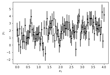
生成模拟数据(\(y = \frac{1}{2}x + 1\)),用高斯噪声产生误差
N = 100
x1 = np.linspace(0, 4, N)
y1 = 0.5*x1 + 1
y1 += np.random.normal(0, 1, size=len(y1))
sigma = 1.
y1_err = np.ones(N)*sigma
画出生成的模拟数据
plt.errorbar(x1, y1, yerr=y1_err,fmt='k.')
plt.xlabel('$x_1$')
plt.ylabel('$y_1$')
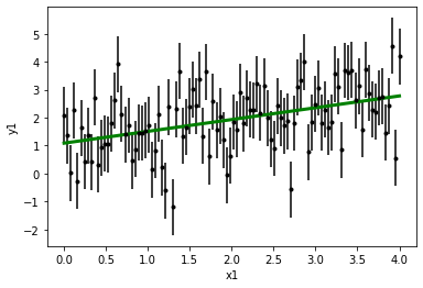
拟合
model = models.Linear1D()
fitter = fitting.LinearLSQFitter()
best_fit = fitter(model, x1, y1, weights=1.0/y1_err**2)
print(best_fit)
Model: Linear1D
Inputs: ('x',)
Outputs: ('y',)
Model set size: 1
Parameters:
    slope            intercept
------------------- -----------------
0.42208417829280787 1.087132048161916
画拟合函数
plt.errorbar(x1,y1,y1_err,fmt='k.')
plt.plot(x1, best_fit(x1), color='g', linewidth=3)
plt.xlabel(r'x1')
plt.ylabel('y1')
二:多项式拟合
导入需要的模块
import numpy as np
import matplotlib.pyplot as plt
from astropy.modeling import models, fitting
from astroquery.vizier import Vizier
import scipy.optimize
# Make plots display in notebooks
%matplotlib inline
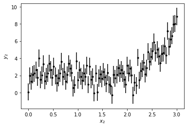
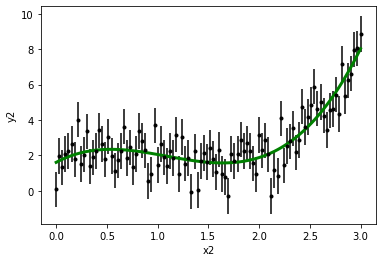
生成模拟数据 (\(y = x^3 - 3x^2 + 2x +2\))
N = 100
x2 = np.linspace(0, 3, N)
y2 = x2**3 - 3*x2**2 + 2*x2 + 2
y2 += np.random.normal(0, 1, size=len(y1))
sigma = 1.
y2_err = np.ones(N)*sigma
画出生成的模拟数据
plt.errorbar(x2, y2, yerr=y2_err,fmt='k.')
plt.xlabel('$x_2$')
plt.ylabel('$y_2$')
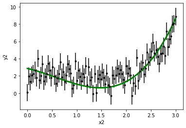
拟合
model_poly = models.Polynomial1D(degree=3)
fitter_poly = fitting.LinearLSQFitter()
best_fit_poly = fitter_poly(model_poly, x2, y2, weights = 1.0/y2_err**2)
print(best_fit_poly)
Model: Polynomial1D
Inputs: ('x',)
Outputs: ('y',)
Model set size: 1
Degree: 3
Parameters:
         c0               c1                 c2                 c3
 ----------------- ---------------- ------------------- ------------------
 1.613139613446467 3.06121833229984 -3.7734605321689005 1.1552346626843524
拟合函数
plt.errorbar(x2,y2,y2_err,fmt='k.')
plt.plot(x2, best_fit_poly(x2), color='g', linewidth=3)
plt.xlabel(r'x2')
plt.ylabel('y2')
another fitter: SimplexLSQFitter
拟合
model_poly = models.Polynomial1D(degree=3)
fitter_poly_2 = fitting.SimplexLSQFitter()
best_fit_poly_2 = fitter_poly_2(model_poly, x2, y2, weights = 1.0/y2_err**2)
print(best_fit_poly_2)
Model: Polynomial1D
Inputs: ('x',)
Outputs: ('y',)
Model set size: 1
Degree: 3
Parameters:
         c0                  c1                  c2                 c3
 ------------------ ------------------- ------------------- ------------------
 2.8684868552438916 -1.2475744910421211 -1.3727224042018307 0.8091486564946109
WARNING: Model is linear in parameters; consider using linear fitting methods. [astropy.modeling.fitting]
WARNING: The fit may be unsuccessful; Maximum number of iterations reached. [astropy.modeling.optimizers]
拟合函数
plt.errorbar(x2,y2,y2_err,fmt='k.')
plt.plot(x2, best_fit_poly_2(x2), color='g', linewidth=3)
plt.xlabel(r'x2')
plt.ylabel('y2')
拟合的统计指标:Reduced Chi Square Value
def calc_reduced_chi_square(fit, x, y, yerr, N, n_free):
    '''
    fit (array) values for the fit
    x,y,yerr (arrays) data
    N total number of points
    n_free number of parameters we are fitting
    '''
    return 1.0/(N-n_free)*sum(((fit - y)/yerr)**2)
第一种拟合的 Reduced Chi Square Value
reduced_chi_squared = calc_reduced_chi_square(best_fit_poly(x2), x2, y2, y2_err, N, 4)
print('Reduced Chi Squared with LinearLSQFitter: {}'.format(reduced_chi_squared))
Reduced Chi Squared with LinearLSQFitter: 0.8378994724726152
第二种拟合的 Reduced Chi Square Value
reduced_chi_squared = calc_reduced_chi_square(best_fit_poly_2(x2), x2, y2, y2_err, N, 4)
print('Reduced Chi Squared with SimplexLSQFitter: {}'.format(reduced_chi_squared))
Reduced Chi Squared with SimplexLSQFitter: 1.3371509473069185
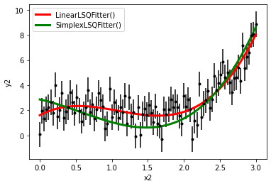
画图
plt.errorbar(x2, y2, yerr=y2_err,fmt='k.')
plt.plot(x2, best_fit_poly(x2), color='r', linewidth=3, label='LinearLSQFitter()')
plt.plot(x2, best_fit_poly_2(x2), color='g', linewidth=3, label='SimplexLSQFitter()')
plt.xlabel(r'x2')
plt.ylabel('y2')
plt.legend()
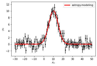
三:高斯拟合
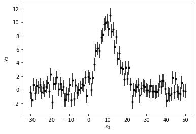
生成模拟数据
mu, sigma, amplitude = 10.0, 5.0, 10.0
N2 = 100
x2 = np.linspace(-30, 50, N)
y2 = amplitude * np.exp(-(x2-mu)**2 / (2*sigma**2))
y2 = np.array([y_point + np.random.normal(0, 1) for y_point in y2])   #Another way to add random gaussian noise
sigma = 1
y2_err = np.ones(N)*sigma
画图
plt.errorbar(x2, y2, yerr=y2_err, fmt='k.')
plt.xlabel('$x_2$')
plt.ylabel('$y_2$')
拟合
model_gauss = models.Gaussian1D()
fitter_gauss = fitting.LevMarLSQFitter()
best_fit_gauss = fitter_gauss(model_gauss, x2, y2, weights=1/y2_err**2)
拟合结果
print(best_fit_gauss)
Model: Gaussian1D
Inputs: ('x',)
Outputs: ('y',)
Model set size: 1
Parameters:
     amplitude             mean              stddev
 ------------------ ------------------ -----------------
 10.052672546272753 10.111106892698416 4.871675460663046
画拟合函数
plt.errorbar(x2, y2, yerr=y2_err, fmt='k.')
plt.plot(x2, best_fit_gauss(x2), 'r-', linewidth=3, label='astropy.modeling')
plt.xlabel('$x_2$')
plt.ylabel('$y_2$')
plt.legend()