
06-NIN 图像分类
NIN网络中,主要提及两点:
1. )多层感知机
2.)global average pooling
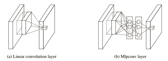
图1 线性卷积层和mlpconv层的区别
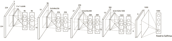
图2 NIN网络架构
第一个卷积核是11x11x3x96,因此在一个patch块上卷积的输出是1x1x96的feature map(一个96维的向量).在其后又接了一个MLP层,输出仍然是96.因此这个MLP层就等价于一个1 x 1 的卷积层,这样工程上任然按照之前的方式实现,不需要额外工作.
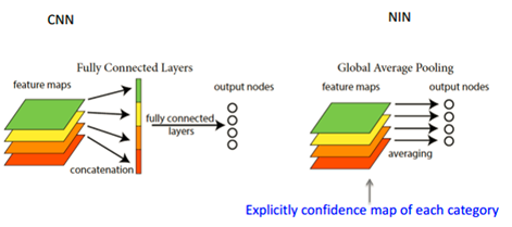
图3 全连接层FC和global average pooling的区别
传统的cnn是在较低层使用卷积,如分类任务中,最后的卷积层所得feature map被矢量化进行全连接层,然后使用softmax 回归进行分类。一般来说,在卷积的末端完成的卷积与传统分类器的桥接。全连接阶段易于过拟合,妨碍整个网络的泛化能力,一般应有一些规则方法来处理过拟合。
在传统CNN中很难解释最后的全连接层输出的类别信息的误差怎么传递给前边的卷积层.而global average pooling更容易解释.另外,全连接层容易过拟合,往往依赖于dropout等正则化手段.
global average pooling的概念非常简单,分类任务有多少个类别,就控制最终产生多少个feature map.对每个feature map的数值求平均作为某类别的置信度,类似FC层输出的特征向量,再经过softmax分类.其优点有:
1.)参数数量减少,减轻过拟合(应用于AlexNet,模型230MB->29MB);
2.)更符合卷积网络的结构,使feature map和类别信息直接映射;
3.)求和取平均操作综合了空间信息,使得对输入的空间变换更鲁棒(与卷积层相连的FC按顺序对特征进行了重新编排(flatten),可能破坏了特征的位置信息).
4.)FC层输入的大小须固定,这限制了网络输入的图像大小.
NIN的pytorch实现:


 1 import torch.nn as nn
 2
 3
 4 #定义模型
 5 class NIN_Net(nn.Module):#继承父类nn.Module
 6     def __init__(self):
 7         super(NIN_Net, self).__init__()#super可以指代父类而不需要显式的声明,这对更改基类(此处为__init__())的时候是有帮助的,使得代码更容易维护
 8         self.classifier = nn.Sequential(
 9                 nn.Conv2d(3, 192, kernel_size=5, stride=1, padding=2),
10                 nn.ReLU(inplace=True),
11                 nn.Conv2d(192, 160, kernel_size=1, stride=1, padding=0),
12                 nn.ReLU(inplace=True),
13                 nn.Conv2d(160,  96, kernel_size=1, stride=1, padding=0),
14                 nn.ReLU(inplace=True),
15                 nn.MaxPool2d(kernel_size=3, stride=2, padding=1),
16                 nn.Dropout(0.5),
17
18                 nn.Conv2d(96, 192, kernel_size=5, stride=1, padding=2),
19                 nn.ReLU(inplace=True),
20                 nn.Conv2d(192, 192, kernel_size=1, stride=1, padding=0),
21                 nn.ReLU(inplace=True),
22                 nn.Conv2d(192, 192, kernel_size=1, stride=1, padding=0),
23                 nn.ReLU(inplace=True),
24                 nn.AvgPool2d(kernel_size=3, stride=2, padding=1),
25                 nn.Dropout(0.5),
26
27                 nn.Conv2d(192, 192, kernel_size=3, stride=1, padding=1),
28                 nn.ReLU(inplace=True),
29                 nn.Conv2d(192, 192, kernel_size=1, stride=1, padding=0),
30                 nn.ReLU(inplace=True),
31                 nn.Conv2d(192,  10, kernel_size=1, stride=1, padding=0),
32                 nn.ReLU(inplace=True),
33                 nn.AvgPool2d(kernel_size=8, stride=1, padding=0),
34
35                 )
36
37     def forward(self, x):
38         x = self.classifier(x)
39
40         #将得到的数据平展
41         x = x.view(x.size(0), 10)
42         return x
classfyNet_main.py
  1 import torch
  2 from torch.utils.data import DataLoader
  3 from torch import nn, optim
  4 from torchvision import datasets, transforms
  5 from torchvision.transforms.functional import InterpolationMode
  6
  7 from matplotlib import pyplot as plt
  8
  9
 10 import time
 11
 12 from Lenet5 import Lenet5_new
 13 from Resnet18 import ResNet18,ResNet18_new
 14 from AlexNet import AlexNet
 15 from Vgg16 import VGGNet16
 16 from Densenet import DenseNet121, DenseNet169, DenseNet201, DenseNet264
 17
 18 from NIN import NIN_Net
 19 from GoogleNet import GoogLeNet
 20
 21 def main():
 22
 23     print("Load datasets...")
 24
 25     # transforms.RandomHorizontalFlip(p=0.5)---以0.5的概率对图片做水平横向翻转
 26     # transforms.ToTensor()---shape从(H,W,C)->(C,H,W), 每个像素点从(0-255)映射到(0-1):直接除以255
 27     # transforms.Normalize---先将输入归一化到(0,1),像素点通过"(x-mean)/std",将每个元素分布到(-1,1)
 28     transform_train = transforms.Compose([
 29                         transforms.Resize((224, 224), interpolation=InterpolationMode.BICUBIC),
 30                         # transforms.RandomCrop(32, padding=4),  # 先四周填充0,在吧图像随机裁剪成32*32
 31                         transforms.RandomHorizontalFlip(p=0.5),
 32                         transforms.ToTensor(),
 33                         transforms.Normalize((0.485, 0.456, 0.406), (0.229, 0.224, 0.225))
 34                     ])
 35
 36     transform_test = transforms.Compose([
 37                         transforms.Resize((224, 224), interpolation=InterpolationMode.BICUBIC),
 38                         # transforms.RandomCrop(32, padding=4),  # 先四周填充0,在吧图像随机裁剪成32*32
 39                         transforms.ToTensor(),
 40                         transforms.Normalize((0.485, 0.456, 0.406), (0.229, 0.224, 0.225))
 41                     ])
 42
 43     # 内置函数下载数据集
 44     train_dataset = datasets.CIFAR10(root="./data/Cifar10/", train=True,
 45                                      transform = transform_train,
 46                                      download=True)
 47     test_dataset = datasets.CIFAR10(root = "./data/Cifar10/",
 48                                     train = False,
 49                                     transform = transform_test,
 50                                     download=True)
 51
 52     print(len(train_dataset), len(test_dataset))
 53
 54     Batch_size = 64
 55     train_loader = DataLoader(train_dataset, batch_size=Batch_size,  shuffle = True, num_workers=4)
 56     test_loader = DataLoader(test_dataset, batch_size = Batch_size, shuffle = False, num_workers=4)
 57
 58     # 设置CUDA
 59     device = torch.device("cuda:0" if torch.cuda.is_available() else "cpu")
 60
 61     # 初始化模型
 62     # 直接更换模型就行,其他无需操作
 63     # model = Lenet5_new().to(device)
 64     # model = ResNet18().to(device)
 65     # model = ResNet18_new().to(device)
 66     # model = VGGNet16().to(device)
 67     # model = DenseNet121().to(device)
 68     # model  = DenseNet169().to(device)
 69
 70     # model = NIN_Net().to(device)
 71
 72     model = GoogLeNet().to(device)
 73
 74     # model = AlexNet(num_classes=10, init_weights=True).to(device)
 75     print(" GoogLeNet train...")
 76
 77     # 构造损失函数和优化器
 78     criterion = nn.CrossEntropyLoss() # 多分类softmax构造损失
 79     # opt = optim.SGD(model.parameters(), lr=0.01, momentum=0.8, weight_decay=0.001)
 80     opt = optim.SGD(model.parameters(), lr=0.01, momentum=0.9, weight_decay=0.0005)
 81
 82     # 动态更新学习率 ------每隔step_size : lr = lr * gamma
 83     schedule = optim.lr_scheduler.StepLR(opt, step_size=10, gamma=0.6, last_epoch=-1)
 84
 85     # 开始训练
 86     print("Start Train...")
 87
 88     epochs = 100
 89
 90     loss_list = []
 91     train_acc_list =[]
 92     test_acc_list = []
 93     epochs_list = []
 94
 95     for epoch in range(0, epochs):
 96
 97         start = time.time()
 98
 99         model.train()
100
101         running_loss = 0.0
102         batch_num = 0
103
104         for i, (inputs, labels) in enumerate(train_loader):
105
106             inputs, labels = inputs.to(device), labels.to(device)
107
108             # 将数据送入模型训练
109             outputs = model(inputs)
110             # 计算损失
111             loss = criterion(outputs, labels).to(device)
112
113             # 重置梯度
114             opt.zero_grad()
115             # 计算梯度,反向传播
116             loss.backward()
117             # 根据反向传播的梯度值优化更新参数
118             opt.step()
119
120             # 100个batch的 loss 之和
121             running_loss += loss.item()
122             # loss_list.append(loss.item())
123             batch_num+=1
124
125
126         epochs_list.append(epoch)
127
128         # 每一轮结束输出一下当前的学习率 lr
129         lr_1 = opt.param_groups[0]['lr']
130         print("learn_rate:%.15f" % lr_1)
131         schedule.step()
132
133         end = time.time()
134         print('epoch = %d/100, batch_num = %d, loss = %.6f, time = %.3f' % (epoch+1, batch_num, running_loss/batch_num, end-start))
135         running_loss=0.0
136
137         # 每个epoch训练结束,都进行一次测试验证
138         model.eval()
139         train_correct = 0.0
140         train_total = 0
141
142         test_correct = 0.0
143         test_total = 0
144
145          # 训练模式不需要反向传播更新梯度
146         with torch.no_grad():
147
148             # print("=======================train=======================")
149             for inputs, labels in train_loader:
150                 inputs, labels = inputs.to(device), labels.to(device)
151                 outputs = model(inputs)
152
153                 pred = outputs.argmax(dim=1)  # 返回每一行中最大值元素索引
154                 train_total += inputs.size(0)
155                 train_correct += torch.eq(pred, labels).sum().item()
156
157
158             # print("=======================test=======================")
159             for inputs, labels in test_loader:
160                 inputs, labels = inputs.to(device), labels.to(device)
161                 outputs = model(inputs)
162
163                 pred = outputs.argmax(dim=1)  # 返回每一行中最大值元素索引
164                 test_total += inputs.size(0)
165                 test_correct += torch.eq(pred, labels).sum().item()
166
167             print("train_total = %d, Accuracy = %.5f %%,  test_total= %d, Accuracy = %.5f %%" %(train_total, 100 * train_correct / train_total, test_total, 100 * test_correct / test_total))
168
169             train_acc_list.append(100 * train_correct / train_total)
170             test_acc_list.append(100 * test_correct / test_total)
171
172         # print("Accuracy of the network on the 10000 test images:%.5f %%" % (100 * test_correct / test_total))
173         # print("===============================================")
174
175     fig = plt.figure(figsize=(4, 4))
176
177     plt.plot(epochs_list, train_acc_list, label='train_acc_list')
178     plt.plot(epochs_list, test_acc_list, label='test_acc_list')
179     plt.legend()
180     plt.title("train_test_acc")
181     plt.savefig('GoogLeNet_acc_epoch_{:04d}.png'.format(epochs))
182     plt.close()
183
184 if __name__ == "__main__":
185
186     main()
