08-模型加速之轻量化模型（二） 深度可分离：MobileNet

　　SqueezeNet虽在一定程度上减少了卷积计算量，但仍然使用传统的卷积计算方式，而在其后的MobileNet利用了更为高效的深度可分离卷积的方式，进一步加速了卷积网络在移动端的应用。

　　为了更好地理解深度可分离卷积，在本节首先回顾标准的卷积计算过程，然后详细讲解深度可分离卷积过程，以及基于此结构的两个网络结构MobileNet v1与MobileNet v2。

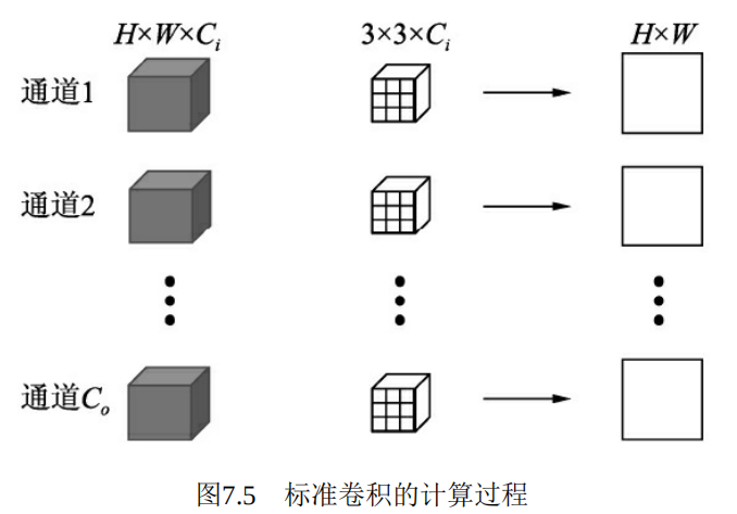
1.）标准卷积

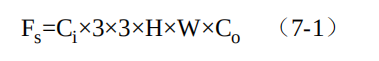
　　假设当前特征图大小为Ci×H×W，需要输出的特征图大小为Co ×H×W，卷积核大小为3×3，Padding为1，则标准卷积的计算过程如图7.5所示。

 

 

 

标准卷积的过程如下：

·对于输入特征图的左上Ci×3×3特征，利用Ci×3×3大小的卷积核进行点乘并求和，得到输出特征图中一个通道上的左上点，这一步操作的计算量为Ci×3×3。

·在输入特征图上进行滑窗，重复第一步操作，最终得到输出特征图中一个通道的H×W大小的输出，总计算量为Ci×3×3×H×W。这一步完成了图7.5中一个通道的过程。

·利用Co个上述大小的卷积核，重复第一步过程，最终得到Co ×H×W大小的特征图。

在整个标准卷积计算过程中，所需的卷积核参数量为Ci×3×3×Co，总的计算量如式（7-1）所示。

需要注意，这里的计算量仅仅是指乘法操作，而没有将加法计算在内。

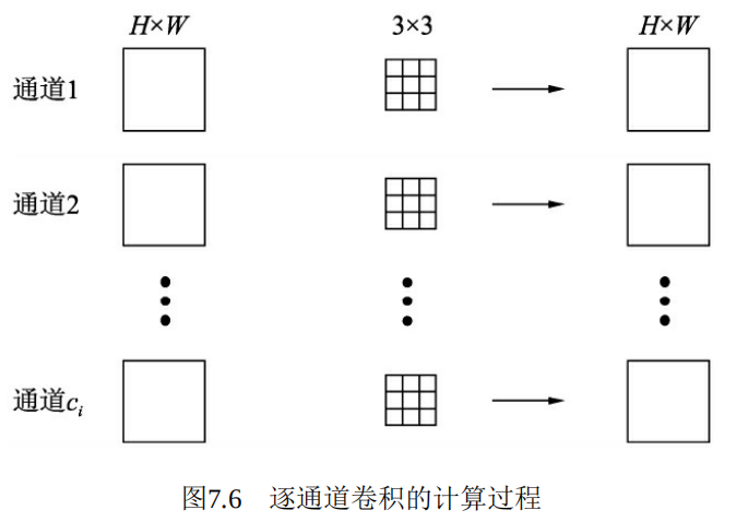
 2.）深度可分离卷积

　　标准卷积在卷积时，同时考虑了图像的区域与通道信息，那么为什么不能分开考虑区域与通道呢？基于此想法，诞生了深度可分离卷积（Depthwise Separable Convolution），将卷积的过程分为逐通道卷积与逐点1×1卷积两步。虽然深度可分离卷积将一步卷积过程扩展为两步，但减少了冗余计算，因此总体上计算量有了大幅度降低。MobileNet也大量采用了深度可分离卷积作为基础单元。

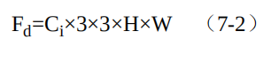
　　逐通道卷积的计算过程如图7.6所示，对于一个通道的输入特征H×W，利用一个3×3卷积核进行点乘求和，得到一个通道的输出H×W。然后，对于所有的输入通道Ci，使用Ci个3×3卷积核即可得到Ci×H×W大小的输出。

　　

 

综合上述计算过程，逐通道卷积有如下几个特点：

·卷积核参数量为Ci×3×3，远少于标准卷积Ci×3×3×Co的数量。

·通道之间相互独立，没有各通道间的特征融合，这也是逐通道积的核心思想，例如图7.6中输出特征的每一个点只对应输入特征一个通道上的3×3大小的特征，而不是标准卷积中Ci×3×3大小。

·由于只在通道间进行卷积，导致输入与输出特征图的通道数相同，无法改变通道数。逐通道卷积的总计算量如式（7-2）所示。

 

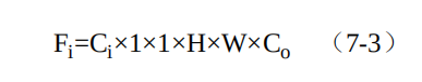
　　由于逐通道卷积通道间缺少特征的融合，并且通道数无法改变，因此后续还需要继续连接一个逐点的1×1的卷积，一方面可以融合不同通道间的特征，同时也可以改变特征图的通道数。由于这里1×1卷积的输入特征图大小为Ci×H×W，输出特征图大小为Co ×H×W，因此这一步的总计算量如式（7-3）所示。

 

　　综合这两步，可以得到深度可分离卷积与标准卷积的计算量之比，如式（7-4）所示。

 

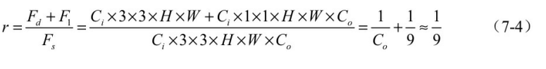
 　　可以看到，虽然深度可分离卷积将卷积过程分为了两步，但凭借其轻量的卷积方式，总体计算量约等于标准卷积的1/9，极大地减少了卷积过程的计算量。

 　　MobileNet v1使用的深度可分离模块的具体结构如图7.7所示。其中使用了BN层及ReLU的激活函数。值得注意的是，在此使用了ReLU6来替代原始的ReLU激活函数，将ReLU的最大输出限制在6以下。

 

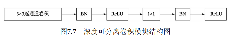
　　 使用ReLU6的原因主要是为了满足移动端部署的需求。移动端通常使用Float16或者Int8等较低精度的模型，如果不对激活函数的输出进行限制的话，激活值的分布范围会很大，而低精度的模型很难精确地覆盖如此大范围的输出，这样会带来精度的损失。

3.）MobileNet v1结构

　　MobileNet v1整体的网络是由上述深度可分离卷积基本单元组成的，具体结构如图7.8所示。与VGGNet类似，也是一个逐层堆叠式网络。图中的Dw代表一个深度分解卷积，其后需要跟一个1×1卷积，s2代表步长为2的卷积，可以缩小特征图尺寸，起到与Pooling层一样的作用.

 

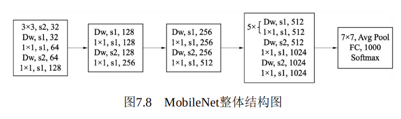
 　　这里列出的是MobileNet v1用于物体分类的网络，可以看到网络最后利用一个全局平均池化层，送入到全连接与Softmax进行分类预测。如果用于物体检测，只需要在之前的特征图上进行特征提取即可。

　　在基本的结构之外，MobileNet v1还设置了两个超参数，用来控制模型的大小与计算量，具体如下：

宽度乘子：用于控制特征图的通道数，记做α，当α＜1时，模型会变得更薄，可以将计算量减少为原来的α 2。

·分辨率乘子：用于控制特征图的尺寸，记做ρ，在相应的特征图上应用该乘子，也可以有效降低每一层的计算量。

　　在实现层面上，PyTorch中卷积层提供了一个组卷积参数，可以方便地实现深度可分离卷积。v>

　　下面利用PyTorch搭建一个MobileNet v1网络，新建一个mobilenet_v1.py，代码如下：

from torch import nn

class  MobileNet(nn.Module):
    
    def __init__(self):
        
        super(MobileNet, self).__init__()
        
        # 标准卷积
        def conv_bn(dim_in, dim_out, stride):
            
            return nn.Sequential(
                nn.Conv2d(dim_in, dim_out, 3, stride, 1, bias=False),
                nn.BatchNorm2d(dim_out),
                nn.ReLU(inplace=True)
            )
        
        # 深度分解卷积
        def conv_dw(dim_in, dim_out, stride):
            
            return nn.Sequential(
                nn.Conv2d(dim_in, dim_in, 3, stride, 1, groups= dim_in, bias=False), # 注：参数groups的使用
                nn.BatchNorm2d(dim_in),
                nn.ReLU(inplace=True),
                nn.Conv2d(dim_in, dim_out, 1, 1, 0, bias=False),
                nn.BatchNorm2d(dim_out),
                nn.ReLU(inplace=True),
            )
        
        self.model = nn.Sequential(
            
            conv_bn(3, 32, 2),
            conv_dw(32, 64, 1),
            conv_dw(64, 128, 2),
            conv_dw(128, 128, 1),
            conv_dw(128, 256, 2),
            conv_dw(256, 256, 1),
            conv_dw(256, 512, 2),
            conv_dw(512, 512, 1),
            conv_dw(512, 512, 1),
            conv_dw(512, 512, 1),
            conv_dw(512, 512, 1),
            conv_dw(512, 512, 1),
            conv_dw(512, 512, 1),
            conv_dw(512, 1024, 2),
            conv_dw(1024, 1024, 1),
            nn.AvgPool2d(7)
        )
        
        self.fc = nn.Linear(1024, 1000)
        
    def forward(self, x):
            
        x = self.model(x)
        x = x.view(-1, 1024)
        x = self.fc(x)
            
        return x   
        

              
                

test_v1.py

import torch
from mobilenet_v1 import MobileNet

mobilenet = MobileNet().cuda()

print(mobilenet)

input = torch.randn(1, 3, 224, 224).cuda()
output  = mobilenet(input)

print(output.shape)

MobileNet(
  (model): Sequential(
    (0): Sequential(
      (0): Conv2d(3, 32, kernel_size=(3, 3), stride=(2, 2), padding=(1, 1), bias=False)
      (1): BatchNorm2d(32, eps=1e-05, momentum=0.1, affine=True, track_running_stats=True)
      (2): ReLU(inplace=True)
    )
    (1): Sequential(
      (0): Conv2d(32, 32, kernel_size=(3, 3), stride=(1, 1), padding=(1, 1), groups=32, bias
      (1): BatchNorm2d(32, eps=1e-05, momentum=0.1, affine=True, track_running_stats=True)
      (2): ReLU(inplace=True)
      (3): Conv2d(32, 64, kernel_size=(1, 1), stride=(1, 1), bias=False)
      (4): BatchNorm2d(64, eps=1e-05, momentum=0.1, affine=True, track_running_stats=True)
      (5): ReLU(inplace=True)
    )
    (2): Sequential(
      (0): Conv2d(64, 64, kernel_size=(3, 3), stride=(2, 2), padding=(1, 1), groups=64, bias
      (1): BatchNorm2d(64, eps=1e-05, momentum=0.1, affine=True, track_running_stats=True)
      (2): ReLU(inplace=True)
      (3): Conv2d(64, 128, kernel_size=(1, 1), stride=(1, 1), bias=False)
      (4): BatchNorm2d(128, eps=1e-05, momentum=0.1, affine=True, track_running_stats=True)
      (5): ReLU(inplace=True)
    )
    (3): Sequential(
      (0): Conv2d(128, 128, kernel_size=(3, 3), stride=(1, 1), padding=(1, 1), groups=128, b
      (1): BatchNorm2d(128, eps=1e-05, momentum=0.1, affine=True, track_running_stats=True)
      (2): ReLU(inplace=True)
      (3): Conv2d(128, 128, kernel_size=(1, 1), stride=(1, 1), bias=False)
      (4): BatchNorm2d(128, eps=1e-05, momentum=0.1, affine=True, track_running_stats=True)
      (5): ReLU(inplace=True)
    )
    (4): Sequential(
      (0): Conv2d(128, 128, kernel_size=(3, 3), stride=(2, 2), padding=(1, 1), groups=128, b
      (1): BatchNorm2d(128, eps=1e-05, momentum=0.1, affine=True, track_running_stats=True)
      (2): ReLU(inplace=True)
      (3): Conv2d(128, 256, kernel_size=(1, 1), stride=(1, 1), bias=False)
      (4): BatchNorm2d(256, eps=1e-05, momentum=0.1, affine=True, track_running_stats=True)
      (5): ReLU(inplace=True)
    )
    (5): Sequential(
      (0): Conv2d(256, 256, kernel_size=(3, 3), stride=(1, 1), padding=(1, 1), groups=256, b
      (1): BatchNorm2d(256, eps=1e-05, momentum=0.1, affine=True, track_running_stats=True)
      (2): ReLU(inplace=True)
      (3): Conv2d(256, 256, kernel_size=(1, 1), stride=(1, 1), bias=False)
      (4): BatchNorm2d(256, eps=1e-05, momentum=0.1, affine=True, track_running_stats=True)
      (5): ReLU(inplace=True)
    )
    (6): Sequential(
      (0): Conv2d(256, 256, kernel_size=(3, 3), stride=(2, 2), padding=(1, 1), groups=256, b
      (1): BatchNorm2d(256, eps=1e-05, momentum=0.1, affine=True, track_running_stats=True)
      (2): ReLU(inplace=True)
      (3): Conv2d(256, 512, kernel_size=(1, 1), stride=(1, 1), bias=False)
      (4): BatchNorm2d(512, eps=1e-05, momentum=0.1, affine=True, track_running_stats=True)
      (5): ReLU(inplace=True)
    )
    (7): Sequential(
      (0): Conv2d(512, 512, kernel_size=(3, 3), stride=(1, 1), padding=(1, 1), groups=512, b
      (1): BatchNorm2d(512, eps=1e-05, momentum=0.1, affine=True, track_running_stats=True)
      (2): ReLU(inplace=True)
      (3): Conv2d(512, 512, kernel_size=(1, 1), stride=(1, 1), bias=False)
      (4): BatchNorm2d(512, eps=1e-05, momentum=0.1, affine=True, track_running_stats=True)
      (5): ReLU(inplace=True)
    )
    (8): Sequential(
      (0): Conv2d(512, 512, kernel_size=(3, 3), stride=(1, 1), padding=(1, 1), groups=512, b
      (1): BatchNorm2d(512, eps=1e-05, momentum=0.1, affine=True, track_running_stats=True)
      (2): ReLU(inplace=True)
      (3): Conv2d(512, 512, kernel_size=(1, 1), stride=(1, 1), bias=False)
      (4): BatchNorm2d(512, eps=1e-05, momentum=0.1, affine=True, track_running_stats=True)
      (5): ReLU(inplace=True)
    )
    (9): Sequential(
      (0): Conv2d(512, 512, kernel_size=(3, 3), stride=(1, 1), padding=(1, 1), groups=512, b
      (1): BatchNorm2d(512, eps=1e-05, momentum=0.1, affine=True, track_running_stats=True)
      (2): ReLU(inplace=True)
      (3): Conv2d(512, 512, kernel_size=(1, 1), stride=(1, 1), bias=False)
      (4): BatchNorm2d(512, eps=1e-05, momentum=0.1, affine=True, track_running_stats=True)
      (5): ReLU(inplace=True)
    )
    (10): Sequential(
      (0): Conv2d(512, 512, kernel_size=(3, 3), stride=(1, 1), padding=(1, 1), groups=512, b
      (1): BatchNorm2d(512, eps=1e-05, momentum=0.1, affine=True, track_running_stats=True)
      (2): ReLU(inplace=True)
      (3): Conv2d(512, 512, kernel_size=(1, 1), stride=(1, 1), bias=False)
      (4): BatchNorm2d(512, eps=1e-05, momentum=0.1, affine=True, track_running_stats=True)
      (5): ReLU(inplace=True)
    )
    (11): Sequential(
      (0): Conv2d(512, 512, kernel_size=(3, 3), stride=(1, 1), padding=(1, 1), groups=512, b
      (1): BatchNorm2d(512, eps=1e-05, momentum=0.1, affine=True, track_running_stats=True)
      (2): ReLU(inplace=True)
      (3): Conv2d(512, 512, kernel_size=(1, 1), stride=(1, 1), bias=False)
      (4): BatchNorm2d(512, eps=1e-05, momentum=0.1, affine=True, track_running_stats=True)
      (5): ReLU(inplace=True)
    )
    (12): Sequential(
      (0): Conv2d(512, 512, kernel_size=(3, 3), stride=(1, 1), padding=(1, 1), groups=512, b
      (1): BatchNorm2d(512, eps=1e-05, momentum=0.1, affine=True, track_running_stats=True)
      (2): ReLU(inplace=True)
      (3): Conv2d(512, 512, kernel_size=(1, 1), stride=(1, 1), bias=False)
      (4): BatchNorm2d(512, eps=1e-05, momentum=0.1, affine=True, track_running_stats=True)
      (5): ReLU(inplace=True)
    )
    (13): Sequential(
      (0): Conv2d(512, 512, kernel_size=(3, 3), stride=(2, 2), padding=(1, 1), groups=512, b
      (1): BatchNorm2d(512, eps=1e-05, momentum=0.1, affine=True, track_running_stats=True)
      (2): ReLU(inplace=True)
      (3): Conv2d(512, 1024, kernel_size=(1, 1), stride=(1, 1), bias=False)
      (4): BatchNorm2d(1024, eps=1e-05, momentum=0.1, affine=True, track_running_stats=True)
      (5): ReLU(inplace=True)
    )
    (14): Sequential(
      (0): Conv2d(1024, 1024, kernel_size=(3, 3), stride=(1, 1), padding=(1, 1), groups=1024
      (1): BatchNorm2d(1024, eps=1e-05, momentum=0.1, affine=True, track_running_stats=True)
      (2): ReLU(inplace=True)
      (3): Conv2d(1024, 1024, kernel_size=(1, 1), stride=(1, 1), bias=False)
      (5): ReLU(inplace=True)
    )
    (15): AvgPool2d(kernel_size=7, stride=7, padding=0)
  )
  (fc): Linear(in_features=1024, out_features=1000, bias=True)
)
torch.Size([1, 1000])

MobileNet v1总结

　　总体上，MobileNet v1利用深度可分离的结构牺牲了较小的精度，带来了计算量与网络层参数的大幅降低，从而也减小了模型的大小，方

便应用于移动端。

　　但MobileNet v1也有其自身结构带来的缺陷，主要有以下两点：

·模型结构较为复古，采用了与VGGNet类似的卷积简单堆叠，没有采用残差、特征融合等先进的结构。

·深度分解卷积中各通道相互独立，卷积核维度较小，输出特征中只有较少的输入特征，再加上ReLU激活函数，使得输出很容易变为0，难以恢复正常训练，因此在训练时部分卷积核容易被训练废掉。

MobileNet v2

针对以上MobileNet v1的缺点，2018年诞生的MobileNet v2吸收了残差网络的思想，主要从两个方面改善了网络结构，提升了MobileNet的检测精度。

首先，MobileNet v2利用残差结构取代了原始的卷积堆叠方式，提出了一个Inverted Residual Block结构，如图7.9所示。依据卷积的步长，该结构可分为两种情形，在步长为1时使用了残差连接，融合的方式为逐元素相加。

相比于MobileNet v1与原始的残差结构，这里有两点不同:

1．Inverted Residual Block结构

　　由于3×3卷积处的计算量较大，因此传统的残差网络通常先使用1×1卷积进行特征降维，减少通道数，再送入3×3卷积，最后再利用1×1卷积

升维。这种结构从形状上看中间窄两边宽，类似于沙漏形状。

　　然而在MobileNet v2中，由于使用了深度可分离卷积来逐通道计算，本身计算量就比较少，因此在此可以使用1×1卷积来升维，在计算量增加不大的基础上获取更好的效果，最后再用1×1卷积降维。这种结构中间宽两边窄，类似于柳叶，该结构也因此被称为Inverted Residual Block。

2．去掉ReLU6

　　深度可分离卷积得到的特征对应于低维空间，特征较少，如果后续接线性映射则能够保留大部分特征，而如果接非线性映射如ReLU，则会破坏特征，造成特征的损耗，从而使得模型效果变差。

　　针对此问题，MobileNet v2直接去掉了每一个Block中最后的ReLU6层，减少了特征的损耗，获得了更好的检测效果。

 

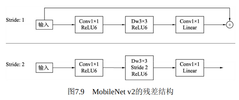
 下面利用PyTorch构建MobileNet v2的残差模块，即图7.9中的stride为1的结构，新建一个mobilenet_v2_block.py文件。代码如下：

from torch import nn

class InvertedResidual(nn.Module):
    
    def __init__(self, inp, oup, stride, expand_ratio):
        
        super(InvertedResidual, self).__init__()
        
        self.stride = stride
        
        hidden_dim =  round(inp*expand_ratio)
        
        self.conv = nn.Sequential(
            #1*1的逐点卷积进行升维
            nn.Conv2d(inp, hidden_dim, 1, 1, 0, bias=False),
            nn.BatchNorm2d(hidden_dim),
            nn.ReLU6(inplace=True),
            
            #深度可分离模块
            nn.Conv2d(hidden_dim, hidden_dim, 3, stride, 1, groups=hidden_dim, bias= False),
            nn.BatchNorm2d(hidden_dim),
            nn.ReLU6(inplace=True),
            
            # 1*1的逐点卷积进行降维
            nn.Conv2d(hidden_dim, oup, 1, 1, 0, bias=False),
            nn.BatchNorm2d(oup)
        )
        
    def forward(self, x):
        return x +self.conv(x)
    

test.py

import torch
from mobilenet_v2_block import InvertedResidual

block = InvertedResidual(24, 24, 1, 6).cuda()
print(block)


input = torch.randn(1, 24, 56, 56).cuda()
output = block(input)
print(output.shape)

InvertedResidual(
  (conv): Sequential(
    (0): Conv2d(24, 144, kernel_size=(1, 1), stride=(1, 1), bias=False)
    (1): BatchNorm2d(144, eps=1e-05, momentum=0.1, affine=True, track_running_stats=True)
    (2): ReLU6(inplace=True)
    (3): Conv2d(144, 144, kernel_size=(3, 3), stride=(1, 1), padding=(1, 1), groups=144, bias=False)
    (4): BatchNorm2d(144, eps=1e-05, momentum=0.1, affine=True, track_running_stats=True)
    (5): ReLU6(inplace=True)
    (6): Conv2d(144, 24, kernel_size=(1, 1), stride=(1, 1), bias=False)
    (7): BatchNorm2d(24, eps=1e-05, momentum=0.1, affine=True, track_running_stats=True)
  )
)
torch.Size([1, 24, 56, 56])

　　总体上，MobileNet v2在原结构的基础上进行了简单的修改，通过较少的计算量即可获得较高的精度，非常适合于移动端的部署。