模型可视化实验笔记
实验基于MVSSNet项目开展:https://github.com/dong03/MVSS-Net
在该论文中,模型整体如下:

ESB部分的四个ResNet输出的图像为:
c1 c2 c3 c4: torch.Size([1, 256, 128, 128]) torch.Size([1, 512, 64, 64]) torch.Size([1, 1024, 32, 32]) torch.Size([1, 2048, 32, 32])
细节一点,边缘检测分支如下:
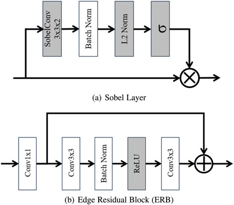
其实这样的设计也不难理解,因为图像篡改部位它无论是边缘还是噪声它都和其他部分不一样,就是很突兀,比如说你把鹿头拼接到狗头上,那么脖子位置的纹理特征肯定是有突变的,同时影响了拼接部分的边缘分布和噪声分布。即使你平滑一下,那也是会留下痕迹的。
1. 可视化特征图:可以看出模型的某一层关注的重点在哪里,在图像分类问题中,意义是看到模型是通过图像的哪一部分来分类的,那么在图像篡改检测问题上,就是发现模型是通过哪个部分来判断图像真假的。
参考帖子 【CNN可视化技术总结(一)--特征图可视化(https://zhuanlan.zhihu.com/p/385858027)】,提到直接可视化。【第七章:PyTorch可视化】(https://blog.csdn.net/qq_36744449/article/details/124639011)
也即对特征图的可视化,一种方法是直接把feature map映射到0-255之间,可以使用torch里面的make_grid函数,但是经过查询,torchvision.utils.make_grid(imgs, padd=2)用途是把多张图像横向拼接而已。
另一种方法是反卷积网络,《Visualizing and Understanding Convolutional Networks》中提出,论文中提出图像像素经过神经网络映射到特征空间,而反卷积网络可以将feature map映射回像素空间。同时还需要用到反池化,类似于反卷积网络的还有一种导向反向传播(论文《Striving for Simplicity:The All Convolutional Net》中提出使用导向反向传播(Guided- backpropagation),导向反向传播与反卷积网络的区别在于对ReLU的处理方式。)。反卷积可以通过tensorboard来做,但是结果看起来有点怪核,也不知意义何在。
于是,我首先尝试第一种方法:
# ---- write at 2023-05-17 18:17
# feature_map[1,3,128,128]
def write_feature_map(feature_map, layer_name):
    feature_map = feature_map.cpu().detach().numpy().squeeze()
    print("feature map origin: ", feature_map.shape)
    if feature_map.ndim == 2:
        feature = np.asarray(feature_map*255, dtype=np.uint8)
        feature = cv2.applyColorMap(feature, cv2.COLORMAP_JET)  # 变成伪彩图
        cv2.imwrite('./CASIAv1-test/save_out/{}-colormap.png'.format(layer_name), feature)
    else:
        feature_map_num = feature_map.shape[0]
        print("feature_map_num: ", feature_map_num)
        for index in range(feature_map_num):
            feature = feature_map[index]
            print("per channel : feature shape: ", feature.shape)
            feature = np.asarray(feature*255, dtype=np.uint8)
            feature = cv2.applyColorMap(feature, cv2.COLORMAP_JET)  # 变成伪彩图
            cv2.imwrite('./CASIAv1-test/save_out/{}-{}-colormap.png'.format(layer_name, index), feature)
特征图这里,我的方法是在原本的模型中,在我需要展示特征图的部分添加一行代码去调用函数,传入特征图,输出其可视化的结果。
对于具有多个通道的三维张量,就全部可视化出来,最后可以看到,比如这个连续四个ResNet,每层ResNet的通道数越来越多,size越来越小,但是其中能够看得懂的特征图比例并不算大,也就是说不是每一个特征图都是有用的,至少对我们人类来说是如此,不是每个特征图都有利于我们对结果进行分类。其实对于我们的模型也是这样,因为在源码里每层都有调用Dropout方法的,模型也会选择性地扔掉一些通道来减小过拟合的程度。
在代码中添加写入特征图的函数:
class MVSSNet(ResNet50):
    def __init__(self, nclass, aux=False, sobel=False, constrain=False, n_input=3, **kwargs):
        super(MVSSNet, self).__init__(pretrained=True, n_input=n_input)
        self.num_class = nclass
        ........
    def forward(self, x):
        size = x.size()[2:]
        input_ = x.clone()
        feature_map, _ = self.base_forward(input_)
        c1, c2, c3, c4 = feature_map
        if self.sobel:
            res1 = self.erb_db_1(run_sobel(self.sobel_x1, self.sobel_y1, c1))
            print("After ERB 1: ", res1.shape)
            write_feature_map(res1, "res1")
            res1 = self.erb_trans_1(res1 + self.upsample(self.erb_db_2(run_sobel(self.sobel_x2, self.sobel_y2, c2))))
            print("After ERB 2: ", res1.shape)
            write_feature_map(res1, "res2")
            res1 = self.erb_trans_2(res1 + self.upsample_4(self.erb_db_3(run_sobel(self.sobel_x3, self.sobel_y3, c3))))
            print("After ERB 3: ", res1.shape)
            write_feature_map(res1, "res3")
            res1 = self.erb_trans_3(res1 + self.upsample_4(self.erb_db_4(run_sobel(self.sobel_x4, self.sobel_y4, c4))), relu=False)
            print("After ERB 4: ", res1.shape)
            write_feature_map(res1, "res4")
然后尝试运行,发现bug:
  File "D:\PythonCVWorkspace\MVSS-Net\models\mvssnet.py", line 349, in forward
    write_feature_map(res1, "res1")
  File "D:\PythonCVWorkspace\MVSS-Net\models\mvssnet.py", line 286, in write_feature_map
    feature_map = feature_map.detach().numpy().squeeze()
TypeError: can't convert cuda:0 device type tensor to numpy. Use Tensor.cpu() to copy the tensor to host memory first.
修改如下:
def write_feature_map(feature_map, name):
    feature_map = feature_map.cpu().detach().numpy().squeeze()
打印出了结果。
在转为伪彩图的时候可能会遇到情况如下:
  File "D:\PythonCVWorkspace\MVSS-Net\models\mvssnet.py", line 303, in write_feature_map
    feature = cv2.applyColorMap(feature, cv2.COLORMAP_JET)  # 变成伪彩图
cv2.error: OpenCV(4.2.0) C:\projects\opencv-python\opencv\modules\imgproc\src\colormap.cpp:714:
    error: (-5:Bad argument) cv::ColorMap only supports source images of type CV_8UC1 or CV_8UC3 in function 'cv::colormap::ColorMap::operator ()'
不过后来发现其实是变量名写错了。
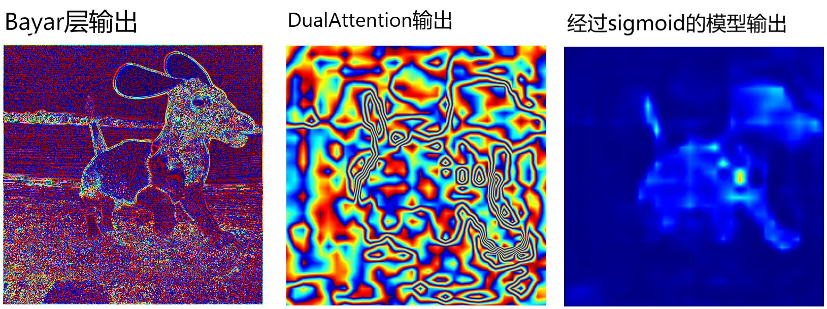
关于Bayar层,它的出处也是一个图像去噪的论文,Bayar是作者的名字,我这里没有贴出,核心在于提出的一个ConstrainedCNN,通过图像的tag来限制卷积核的输出的分布,论文提出是这样做便可以检测出高频特征,也就是噪声,然后我打印出了Bayar层的特征图,确实看得出,我们拿出它每一个局部,都是一个纹理特征,不过看起来更像是许许多多的噪点构成的纹理。不知这个可视化结果能不能佐证原论文的说法,但是相比于我们在ResNet中输出的特征图来看,确实有很大不同。但是这样的特征图在经过ResNet之后,所得到的特征图至少我们肉眼看来和ESB分支没有很大的不同,不过从模型设计上看,一个检测边缘,一个侧重于高频分量,也许这个就无法从特征图上体现出来吧。
输出特征图如下:
2. CAM(Class Activation Map)类激活。
原理参考:
类激活图(CAM)代码+原理详解【pytorch亲测有效】(https://blog.csdn.net/qq_44722174/article/details/117000910)
- 经过全局平均池化(GAP),512张特征图被降维为长度512的特征向量
- 最后,特征向量与权重矩阵W点积,再经过softmax函数压缩为[0,1]区间内的概率
其实做GAP的目的,无非就是得到每一个通道的权重,如果我们没有全连接层的话,直接把特征图做全局平均池化然后通过Softmax得到概率作为权重就可以了,甚至如果我们是二分类的话,直接做Sigmoid也是可以的,但是做加权求和的时候还是需要归一化一下,让权重之和为1,这样我们叠加到原图像上的效果看起来才好看。否则权重太小了看着不明显,权重太大了原图看不清。
同直接可视化一样,CAM系列也不需要重新训练也不需要改变模型结构。
查到了很多Grad-CAM的帖子,或者Grad-CAM++,包括CAM方法,都要求全连接层以及Softmax的类别信息,然后根据类别信息对特征图求梯度。
通过查看模型结构,找到几个位置可能有用的:
两个ResNet最后都有池化层和全连接层、两个Attention结构都有Softmax层。
  (res50): ResNet50(
    (model): ResNet(
......略......
      (maxpool): MaxPool2d(kernel_size=3, stride=2, padding=1, dilation=1, ceil_mode=False)
      (layer1): Sequential(
......略......
      )
      (avgpool): AvgPool2d(kernel_size=7, stride=1, padding=0)
      (fc): Linear(in_features=2048, out_features=1000, bias=True)
    )
    (relu): ReLU(inplace=True)
  )
......略......
    (pam): _PositionAttentionModule(
      (conv_b): Conv2d(1024, 128, kernel_size=(1, 1), stride=(1, 1))
      (conv_c): Conv2d(1024, 128, kernel_size=(1, 1), stride=(1, 1))
      (conv_d): Conv2d(1024, 1024, kernel_size=(1, 1), stride=(1, 1))
      (softmax): Softmax(dim=-1)
    )
    (cam): _ChannelAttentionModule(
      (softmax): Softmax(dim=-1)
    )
但我暂时没有找到代码中关于分类的程序也没找到Softmax计算的代码。因此放弃Grad-CAM,看看单纯的CAM如何实现。
通过如下代码,打印深度网络的每一层,从而可以通过key来获取权重:
for key in model.state_dict().keys():
    print(key)
例如,如此获取某一层的权重tensor数据:
keys = model.state_dict().keys()
model.state_dict()["model.fc.weight"]
打印:
tensor([[-0.0092,  0.0153, -0.0375,  ..., -0.0105,  0.0011, -0.0265],
        [ 0.0104, -0.0266,  0.0005,  ...,  0.0288, -0.0210, -0.0067],
        ...,
        [-0.0215,  0.0239,  0.0809,  ...,  0.0010, -0.0440,  0.0180]],
       device='cuda:0'
不过CAM关键是求出特征图每一个像素的所属类别,因此不一定要找到Softmax函数,只需要看看自己研究的模型,它在输出结果之前做了什么变换,
例如MVSSNet的架构中,输出了黑白蒙版,是在DualAttention和Sigmoid之后,因此这里由DualAttention输出特征图,由Sigmoid做分类,因此可以在这里做CAM。
首先在inference函数里面找到调用模型的地方:
def inference_single(img, model, th=0):
    model.eval()
    with torch.no_grad():
        img = img.reshape((-1, img.shape[-3], img.shape[-2], img.shape[-1]))
        img = direct_val(img)
        img = img.cuda()
        _, seg_feat = run_model(model, img)
        seg = torch.sigmoid(seg_feat).detach().cpu()
        # ----可见,上面运行模型的一次推理,然后输出最终的mask,而且刚好在sigmoid之前----
        # ----刚好符合我们的需求,编写函数绘制CAM
        get_cam(seg)
        ......略......
    return fake_seg, max_score
然后是CAM函数:
def get_cam(cam):
    cam = cam.squeeze()
    cam_img = (cam - cam.min()) / (cam.max() - cam.min())
    cam_img = np.uint8(255 * cam_img)
    img = cv2.imread("./CASIAv1-test/TP/Sp/1abo79_c8vzcuv_0.jpg")
    height, width, _ = img.shape  #读取输入图片的尺寸
    heatmap = cv2.applyColorMap(cv2.resize(cam_img, (width, height)), cv2.COLORMAP_JET)  #CAM resize match input image size
    result = heatmap * 0.5 + img * 0.5    #两张图片相加的比例
    CAM_RESULT_PATH = './CASIAv1-test/save_out/'   #把结果存下来
    cv2.imwrite(CAM_RESULT_PATH + "cam-res-0.png", result)  #存储
然后运行一下整个模型的推理,推理当中就会调用该函数,结果如图所示:
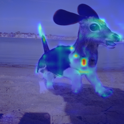
事实上我还做过一个尝试,就是对ResNet层的特征图绘制CAM,得到的效果就是,图片中这只狗的全身对应位置的热力图颜色是橙黄色到红色,当然脖子位置红色很明显,其他背景图位置是绿色到黄绿色。那其实和这个图片比较像,只是暂时只关注到了图像中的主体,但还没关注到篡改位置在脖子部分,之后经过几次边缘检测分支的迭代,也就是Sobel算子ERB模块,加上NRB分支和双注意力模块,才看到了脖子部分的不同。
但毕竟效果不清楚,接下来尝试一下pytorch-grad-cam库
pip install grad-cam -i http://pypi.douban.com/simple/ --trusted-host pypi.douban.com
提取层的办法:
resn = list(model.children())
# ERB
# for i in range(4, 11):
#     print(resn[i])
# ResNet1
# print(resn[19])
# Bayar
# print(resn[20])
# DAHead
# print(resn[21])
dahead = list(resn[21].children())
print(dahead[2])
print(dahead[3])
print(dahead[6])
# print(list(resn.children()))

output:
_PositionAttentionModule(
  (conv_b): Conv2d(1024, 128, kernel_size=(1, 1), stride=(1, 1))
  (conv_c): Conv2d(1024, 128, kernel_size=(1, 1), stride=(1, 1))
  (conv_d): Conv2d(1024, 1024, kernel_size=(1, 1), stride=(1, 1))
  (softmax): Softmax(dim=-1)
)
_ChannelAttentionModule(
  (softmax): Softmax(dim=-1)
)
Sequential(
  (0): Dropout(p=0.1, inplace=False)
  (1): Conv2d(1024, 1, kernel_size=(1, 1), stride=(1, 1))
)
如今我有个疑问,如果不是连接了激活函数的层,也能做Grad-CAM吗?
再安装flashtorch来做可视化试一试,不过仍然失败了,给的案例参考价值不大。
再试一试tensorboard,需要注意的是,pytorch要使用tensorboard需要安装tensorflow,以及tensorflow自带的tensorboard。
-
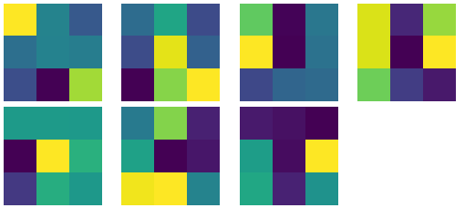
可视化卷积核
可视化卷积核首先查看模型结构:
print(len(model.state_dict().keys()))
for key in model.state_dict().keys():
    print(key)

output:
800
model.conv1.weight
model.bn1.weight
model.bn1.bias
......略......
head.out.1.weight
head.out.1.bias
然后拿出自己想要可视化参数的层,绘图
kernels = []
kernels.append(model.state_dict()["erb_db_1.conv3.weight"])
kernels.append(model.state_dict()["erb_db_2.conv3.weight"])
kernels.append(model.state_dict()["erb_db_3.conv3.weight"])
kernels.append(model.state_dict()["erb_db_4.conv3.weight"])
kernels.append(model.state_dict()["erb_trans_1.conv3.weight"])
kernels.append(model.state_dict()["erb_trans_2.conv3.weight"])
kernels.append(model.state_dict()["erb_trans_3.conv3.weight"])

plt.figure(0)
for i in range(len(kernels)):
    plt.subplot(2, 4, i+1)
    plt.axis('off')
    plt.imshow(kernels[i].squeeze().cpu().detach())
plt.show()
以上七个卷积核都是3×3的,结果如下:
---