图像处理-图像增强（空域）笔记

目录：Histogram、Equalization、CLAHE、......

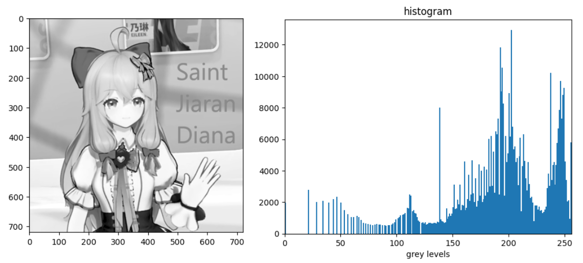
Image Histograms: The histogram of an image shows us the distribution of grey levels in the image.

import numpy as np
import matplotlib.pyplot as plt
import cv2

img_path = "../img-input/diana-221116-square-text.png"
img = cv2.imread(img_path, cv2.IMREAD_GRAYSCALE)  # read gray image

# plot grey RGB image.
# plt.figure(0)
# img_grey_rgb = cv2.cvtColor(img, cv2.COLOR_BGR2RGB)
# plt.imshow(img_grey_rgb)
# plt.show()

plt.figure(1)
plt.hist(img.ravel(), 256, [0, 256])
plt.xlabel("grey levels")
plt.title("histogram")
plt.xlim([0, 256])
plt.show()

output:

Histogram Equalization

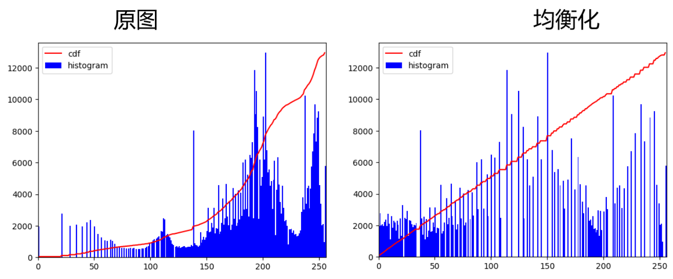
A good image will have pixels from all regions of the image.

参考opencv官方文档的手动均衡化方法：

# 原图
def plot_hist(img):
    hist, bins = np.histogram(img.flatten(), 256, [0, 256])
    cdf = hist.cumsum()
    cdf_normalized = cdf * float(hist.max()) / cdf.max()
    plt.figure(4)
    plt.plot(cdf_normalized, color = 'r')
    plt.hist(img.flatten(),256,[0,256], color = 'b')
    plt.xlim([0,256])
    plt.legend(('cdf','histogram'), loc = 'upper left')
    plt.show()
plot_hist(img)
# 均衡化
hist, bins = np.histogram(img.flatten(), 256, [0, 256])
cdf = hist.cumsum()
cdf_m = np.ma.masked_equal(cdf, 0)
cdf_m = (cdf_m - cdf_m.min())*255/(cdf_m.max()-cdf_m.min())
cdf = np.ma.filled(cdf_m,0).astype('uint8')
img2 = cdf[img]
plot_hist(img2)

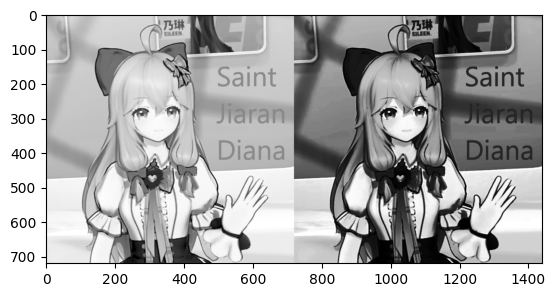
另一种方法是，opencv里封装的函数直接调用，一行代码，和上面的手动的代码最终效果一模一样：

equ = cv2.equalizeHist(img)
res = np.hstack((img, equ))
res_grey_rgb = cv2.cvtColor(res, cv2.COLOR_BGR2RGB)
plt.figure(5)
plt.imshow(res_grey_rgb)
plt.show()

如图：左侧为原图，右侧为均衡化后的效果。

CLAHE Contrast Limited Adaptive Histogram Equalization

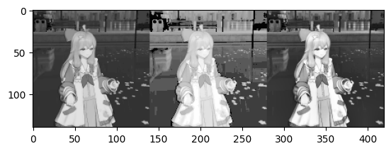
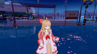
CLAHE的技术背景：以上方法并非总是起作用，加入图像由前景和背景组成，如下图，那么不同部分的色度、亮度、饱和度都会互相影响：

均衡化结果如下，背景确实质量更好了，细节更显得丰富，但是前景却被过曝(over-brightness)：

So to solve this problem, adaptive histogram equalization is used. In this, image is divided into small blocks called "tiles" (tileSize is 8x8 by default in OpenCV). Then each of these blocks are histogram equalized as usual.

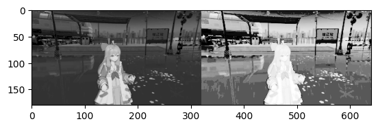
# ==========CLAHE============
import numpy as np
import matplotlib.pyplot as plt
import cv2
# ----------------read------------
img_path = "../img-input/station-140.png"

img = cv2.imread(img_path, cv2.IMREAD_GRAYSCALE)  # read gray image
# ==========未经CLAHE处理的结果========
equ = cv2.equalizeHist(img)

# plt.figure(6)
# plt.imshow(res_grey_rgb)
# plt.show()
# CLAHE
clahe = cv2.createCLAHE(clipLimit=2.0, tileGridSize=(8,8))
cla = clahe.apply(img)

res = np.hstack((img, equ, cla))
res_grey_rgb = cv2.cvtColor(res, cv2.COLOR_BGR2RGB)
plt.figure(6)
plt.imshow(res_grey_rgb)
cv2.imwrite("../img-output/claheres.png", res_grey_rgb)

结果如下三个图分别是 原图、equalization、CLAHE，也许是选图不好，CLAHE效果不是那么地明显，不过看得出背景更清晰、人物更饱和：