c.Matlab(数据和函数的可视化)
A.二维曲线绘图的基本操作
1.plot基本调用格式

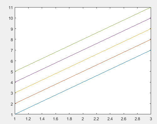
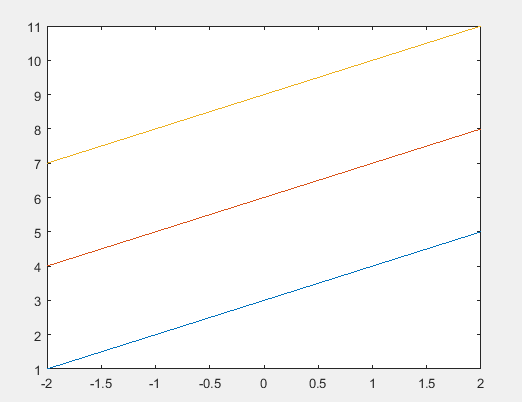
close all;
x=[1,2,3,4,5;4,5,6,7,8;7,8,9,10,11];%生成随机整数矩阵,大小为5X3,范围在1-10中
y=(-2:2)';
figure,plot(x);%x矩阵有5列,所以有五条线,每列三个值,把这三个数连起来,列数为自变量,每一列对应的所有元素元素为因变量
figure,plot(y,x);%y为自变量,y的元素个数等于x的列数,x的每一行为因变量
figure,plot(x,y);%x为二维数组,y为向量,x的每一列为自变量,y的元素为因变量
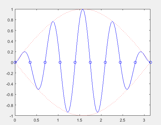
2.用图形表示连续调制波形及其包络线
t=(0:pi/100:pi)'; %长度为101的时间采样列向量
y1=sin(t)*[1,-1]; %包络线函数值,是(101x2)的矩阵
y2=sin(t).*sin(9*t); %长度为101的调制波列向量
t3=pi*(0:9)/9;%过零点
y3=sin(t3).*sin(9*t3);
plot(t,y1,'r:',t,y2,'b',t3,y3,'bo')
% plot(t,y1,'r:')
% hold on
% plot(t,y2,'b')
% plot(t3,y3,'bo')
%hold off
axis([0,pi,-1,1]) %控制轴的范围
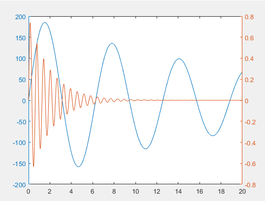
3.双纵坐标
x = 0:0.01:20;
y1 = 200*exp(-0.05*x).*sin(x);
y2 = 0.8*exp(-0.5*x).*sin(10*x);
figure,plotyy(x,y1,x,y2)
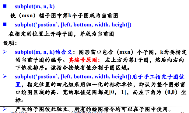
B.多子图
close all
t=(pi*(0:1000)/1000)';
y1=sin(t);y2=sin(10*t);y12=sin(t).*sin(10*t);
subplot(2,2,1),plot(t,y1);axis([0,pi,-1,1])
subplot(2,2,2),plot(t,y2);axis([0,pi,-1,1])
subplot('position',[0.2,0.05,0.6,0.45])
% 假设整个图形窗口长宽都是1
% [0.2,0.05,0.6,0.45]
%0.2表示图像离最左端的距离为0.2
% 0.05表示图像离底端的距离为0.05
% 0.6表示图像的宽为0.6
% 0.45表示图像的高为0.45
plot(t,y12,'b-',t,[y1,-y1])

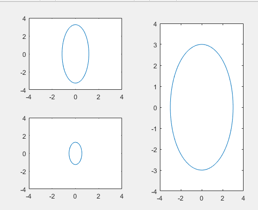
t=0:pi/100:2*pi;
x1=1.15*cos(t);
y1=3.25*sin(t);
x2=0.55*cos(t);
y2=1.25*sin(t);
x3=3*cos(t);
y3=3*sin(t);
subplot(2,2,1),plot(x1,y1),axis([-4 4 -4 4]);
subplot(2,2,3),plot(x2,y2),axis([-4 4 -4 4]);
subplot('position',[0.6,0.1,0.3,0.8]),plot(x3,y3),axis([-4 4 -4 4]);
C.辅助画图
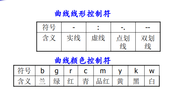
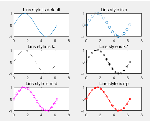
1,线形,颜色,点形

t=(0:15)*2*pi/15;
% 0到2pi范围内有十五个点,想改几个点改几个点
y=sin(t);
subplot(3,2,1), plot(t, y); title('Lins style is default')
% 默认是蓝色的实线,实点
subplot(3,2,2), plot(t, y, 'o'); title('Lins style is o')
% 蓝色的点,不写线形的话就没线
subplot(3,2,3), plot(t, y, 'k:'); title('Lins style is k:')
% 黑色的,虚线,没点
subplot(3,2,4), plot(t, y, 'k:*'); title('Lins style is k:*')
% 黑色,虚线,点用*点描
subplot(3,2,5), plot(t, y, 'm-d'); title('Lins style is m-d')
% 点是菱形品红色,用实线连起来
subplot(3,2,6), plot(t, y, 'r-p'); title('Lins style is r-p')
% 红色,实线,五角星符号
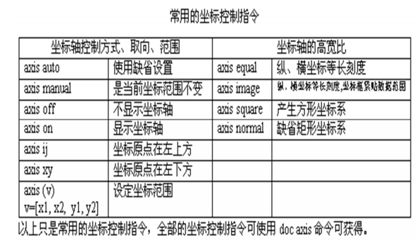
2.坐标控制
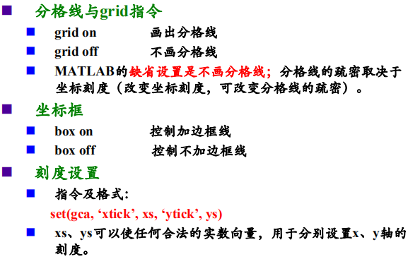
3.刻度、分割线、坐标框
t=6*pi*(0:100)/100; %等效于[0:1/100:1]*6*pi 0~6pi
y=1-exp(-0.3*t).*cos(0.7*t);
tt=t(abs(y-1)>0.05); %y值在-0.95~1.05区间外的点
% tt=t(find(abs(y-1)>0.05))
ts=max(tt); %何时收敛
plot(t,y,'r-');
grid on;
axis([0, 6*pi,0.6,max(y)]);
% 坐标轴范围
title('y=1-exp(-\alpha*t)*cos(\omega*t)');
hold on;
yts=1-exp(-0.3*ts).*cos(0.7*ts);
plot(ts,yts,'bo');
% 标出收敛的点
hold off;
set(gca,'xtick',[2*pi,4*pi,6*pi],'ytick',[0.95,1,1.05,max(y)]);
% 刻度设置
grid on;
% 画出分割线

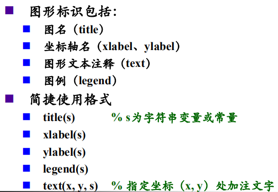
4.图形标识
a、基本图形标识
b、字体形式设置

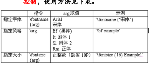
例1
t=(0:100)/100*2*pi;
y=sin(t);
plot(t, y)
text(3*pi/4,sin(3*pi/4), '\fontsize{16}\leftarrowsin(t) = .707 ')
% 16号字体,左箭头,要写的东西
text(pi, sin(pi), '\fontsize{16}\leftarrowsin(t) = 0 ')
text(5*pi/4, sin(5*pi/4), '\fontsize{16}sin(t) = -.707\rightarrow',...
'HorizontalAlignment','right')%设置图形标识为水平右对齐,默认左对齐
例2
t = 0:900;
plot(t,0.25*exp(-0.005*t))
title('\fontsize{16}\itAe^{\alphat}');
text(300,.25*exp(-0.005*300),...
    '\fontsize{14}\leftarrow0.25\ite^-0.005\itt at \itt = 300');
%      14号字体    左箭头再写0.25 斜体写e^-0.005t at t=300
% text(300,.25*exp(-0.005*300),...
%     '\fontsize{14}\leftarrow0.25\ite^-0.005t at t = 300');

D.特殊图形
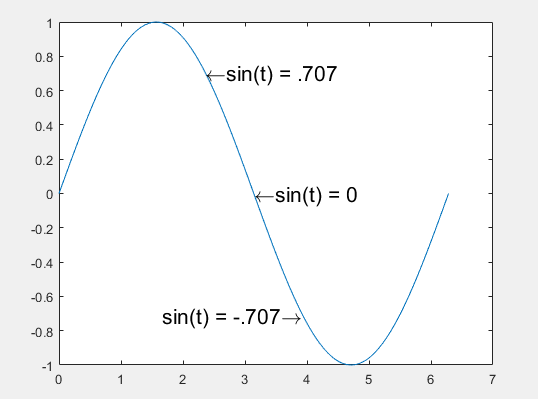
1.直方图
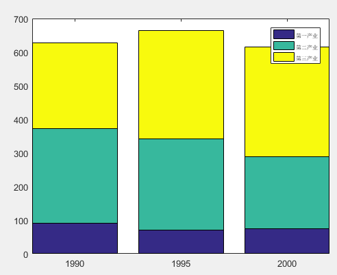
a.累计式直方图
x = -2.9:0.2:2.9;
bar(x,exp(-x.*x),'r')
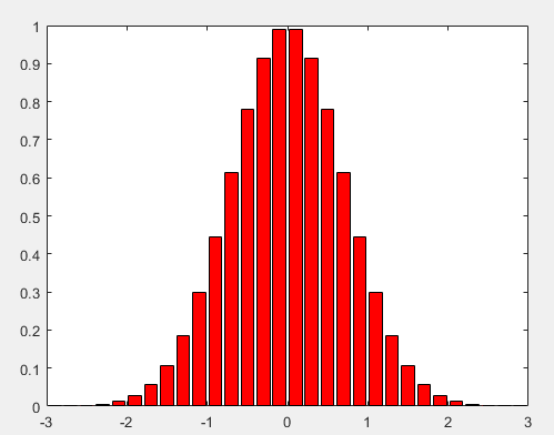
year=[1990 1995 2000];
people=[90.7 281.6 254.8; 70.6 271 323.7; 73.9 214.6 326.5];
bar(year, people, 'stack');
%barh(year, people, ‘stack’); % 横向累积式直方图
legend('\fontsize{6}第一产业', '\fontsize{6}第二产业', '\fontsize{6}第三产业');
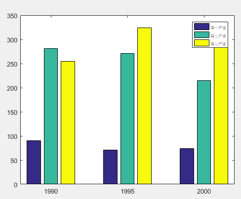
b.分组式直方图
year=[1990 1995 2000];
people=[90.7 281.6 254.8; 70.6 271 323.7; 73.9 214.6 326.5];
bar(year, people, 'group'); % 分组式直方图
%barh(year, people, ‘group’); % 横向分组式直方图
legend('\fontsize{6}第一产业’, ‘\fontsize{6}第二产业’, ‘\fontsize{6}第三产业')
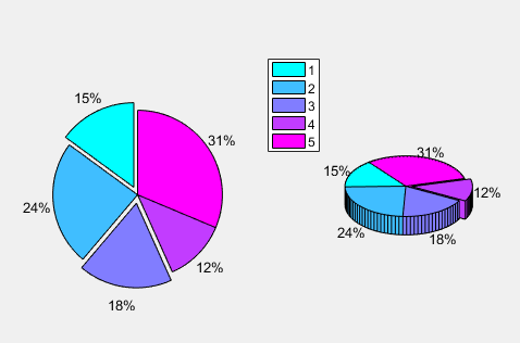
2.饼状图
a=[1,1.6,1.2,0.8,2.1];
subplot(1,2,1),pie(a,[1 0 1 0 0]),% 1对应的部分会突出
legend({'1','2','3','4','5'})
subplot(1,2,2), b=int8(a==min(a));
% a是否是最小的,是的话b取1,生成一个布尔型的矩阵,int8强制转换成数据型
pie3(a,b)% 突出b这一部分
colormap(cool)
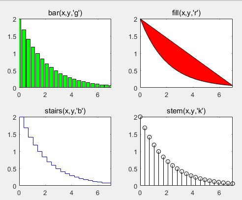
3.各种图
x = 0:0.35:7;
y = 2*exp(-0.5*x);
subplot(2,2,1);bar(x,y,'g');
% subpolt没逗号也可以,但是要养成好习惯
title('bar(x,y,''g'')');axis([0,7,0,2]);% 条形图
subplot(222);fill(x,y,'r');
title('fill(x,y,''r'')');axis([0,7,0,2]);%填充图
subplot(223);stairs(x,y,'b');
title('stairs(x,y,''b'')');axis([0,7,0,2]);% 阶梯图
subplot(224);stem(x,y,'k');
title('stem(x,y,''k'')');axis([0,7,0,2]);% 离散杆图
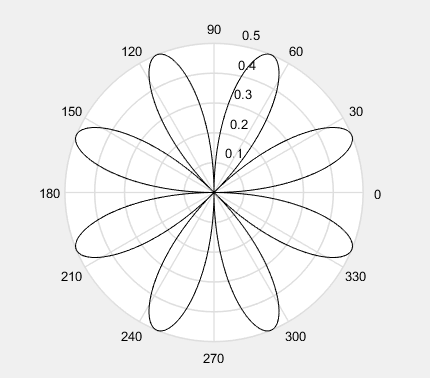
4.极坐标图
theta = 0:0.01:2*pi;
rho = sin(2*theta).*cos(2*theta);
polar(theta,rho,'k');
% 极坐标自动会加网格线,与xy坐标不同
E.三维图
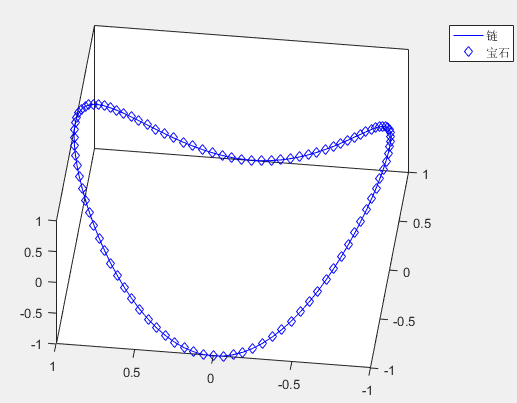
1.三维线图
t=(0:0.02:2)*pi;
x=sin(t);
y=cos(t);
z=cos(2*t);
plot3(x,y,z,'b-',x,y,z,'bd');
% 先画蓝色的实线,再画蓝色的菱形线,菱形在点上
view([-83,58]);
% 规定看的视角,方位角逆时针转的角度是负的,俯仰角
box on
%长方体的边边
legend('链','宝石')
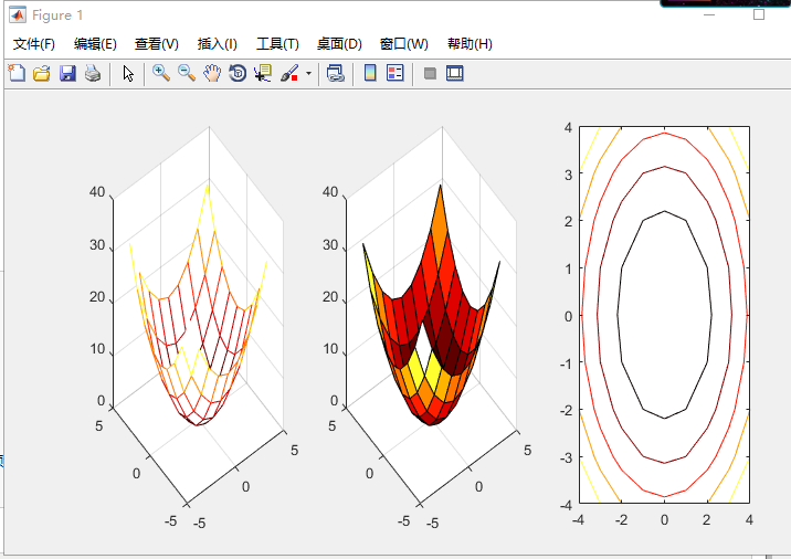
2.网线图,曲面图,等高线
x=-4:4;y=x;
[xa,ya]=meshgrid(x,y); %生成 x-y 坐标“格点”矩阵
% x取-4到4(9个数),y取-4(9个数),这样可以画出一条线
% x取-4到4(9个数),y取-3(9个数),这样可以画出第二条线
%有九条线
z=xa.^2+ya.^2; %计算格点上的函数值
subplot(1,3,1), mesh(x,y,z); %三维网格图
subplot(1,3,2), surf(x,y,z); %三维曲面图
subplot(1,3,3), contour(x,y,z); %等高线,高的颜色亮,低的颜色深
colormap(hot);