Hacker's guide to Neural Networks - 4

from  http://karpathy.github.io/neuralnets/

previous: https://www.cnblogs.com/zhangzhiwei122/p/15887335.html 

 

Example: Single Neuron

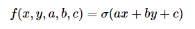
In the previous section you hopefully got the basic intuition behind backpropagation. Lets now look at an even more complicated and borderline practical example. We will consider a 2-dimensional neuron that computes the following function:

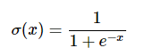
In this expression, σσ is the sigmoid function. Its best thought of as a “squashing function”, because it takes the input and squashes it to be between zero and one: Very negative values are squashed towards zero and positive values get squashed towards one. For example, we have sig(-5) = 0.006, sig(0) = 0.5, sig(5) = 0.993. Sigmoid function is defined as:

The gradient with respect to its single input, as you can check on Wikipedia or derive yourself if you know some calculus is given by this expression:

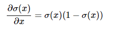
For example, if the input to the sigmoid gate is x = 3, the gate will compute output f = 1.0 / (1.0 + Math.exp(-x)) = 0.95, and then the (local) gradient on its input will simply be dx = (0.95) * (1 - 0.95) = 0.0475.

That’s all we need to use this gate: we know how to take an input and forward it through the sigmoid gate, and we also have the expression for the gradient with respect to its input, so we can also backprop through it. Another thing to note is that technically, the sigmoid function is made up of an entire series of gates in a line that compute more atomic functions: an exponentiation gate, an addition gate and a division gate. Treating it so would work perfectly fine but for this example I chose to collapse all of these gates into a single gate that just computes sigmoid in one shot, because the gradient expression turns out to be simple.

Lets take this opportunity to carefully structure the associated code in a nice and modular way. First, I’d like you to note that every wire in our diagrams has two numbers associated with it:

1. the value it carries during the forward pass
2. the gradient (i.e the pull) that flows back through it in the backward pass

Lets create a simple Unit structure that will store these two values on every wire. Our gates will now operate over Units: they will take them as inputs and create them as outputs.

// every Unit corresponds to a wire in the diagrams
var Unit = function(value, grad) {
  // value computed in the forward pass
  this.value = value; 
  // the derivative of circuit output w.r.t this unit, computed in backward pass
  this.grad = grad; 
}

In addition to Units we also need 3 gates: +, * and sig (sigmoid). Lets start out by implementing a multiply gate. I’m using Javascript here which has a funny way of simulating classes using functions. If you’re not a Javascript - familiar person, all that’s going on here is that I’m defining a class that has certain properties (accessed with use of this keyword), and some methods (which in Javascript are placed into the function’s prototype). Just think about these as class methods. Also keep in mind that the way we will use these eventually is that we will first forward all the gates one by one, and then backward all the gates in reverse order. Here is the implementation:

var multiplyGate = function(){ };
multiplyGate.prototype = {
  forward: function(u0, u1) {
    // store pointers to input Units u0 and u1 and output unit utop
    this.u0 = u0; 
    this.u1 = u1; 
    this.utop = new Unit(u0.value * u1.value, 0.0);
    return this.utop;
  },
  backward: function() {
    // take the gradient in output unit and chain it with the
    // local gradients, which we derived for multiply gate before
    // then write those gradients to those Units.
    this.u0.grad += this.u1.value * this.utop.grad;
    this.u1.grad += this.u0.value * this.utop.grad;
  }
}

The multiply gate takes two units that each hold a value and creates a unit that stores its output. The gradient is initialized to zero. Then notice that in the backward function call we get the gradient from the output unit we produced during the forward pass (which will by now hopefully have its gradient filled in) and multiply it with the local gradient for this gate (chain rule!). This gate computes multiplication (u0.value * u1.value) during forward pass, so recall that the gradient w.r.t u0 is u1.value and w.r.t u1 is u0.value. Also note that we are using += to add onto the gradient in the backward function. This will allow us to possibly use the output of one gate multiple times (think of it as a wire branching out), since it turns out that the gradients from these different branches just add up when computing the final gradient with respect to the circuit output. The other two gates are defined analogously:

var addGate = function(){ };
addGate.prototype = {
  forward: function(u0, u1) {
    this.u0 = u0; 
    this.u1 = u1; // store pointers to input units
    this.utop = new Unit(u0.value + u1.value, 0.0);
    return this.utop;
  },
  backward: function() {
    // add gate. derivative wrt both inputs is 1
    this.u0.grad += 1 * this.utop.grad;
    this.u1.grad += 1 * this.utop.grad;
  }
}

var sigmoidGate = function() { 
  // helper function
  this.sig = function(x) { return 1 / (1 + Math.exp(-x)); };
};
sigmoidGate.prototype = {
  forward: function(u0) {
    this.u0 = u0;
    this.utop = new Unit(this.sig(this.u0.value), 0.0);
    return this.utop;
  },
  backward: function() {
    var s = this.sig(this.u0.value);
    this.u0.grad += (s * (1 - s)) * this.utop.grad;
  }
}

Note that, again, the backward function in all cases just computes the local derivative with respect to its input and then multiplies on the gradient from the unit above (i.e. chain rule). To fully specify everything lets finally write out the forward and backward flow for our 2-dimensional neuron with some example values:

// create input units
var a = new Unit(1.0, 0.0);
var b = new Unit(2.0, 0.0);
var c = new Unit(-3.0, 0.0);
var x = new Unit(-1.0, 0.0);
var y = new Unit(3.0, 0.0);

// create the gates
var mulg0 = new multiplyGate();
var mulg1 = new multiplyGate();
var addg0 = new addGate();
var addg1 = new addGate();
var sg0 = new sigmoidGate();

// do the forward pass
var forwardNeuron = function() {
  ax = mulg0.forward(a, x); // a*x = -1
  by = mulg1.forward(b, y); // b*y = 6
  axpby = addg0.forward(ax, by); // a*x + b*y = 5
  axpbypc = addg1.forward(axpby, c); // a*x + b*y + c = 2
  s = sg0.forward(axpbypc); // sig(a*x + b*y + c) = 0.8808
};
forwardNeuron();

console.log('circuit output: ' + s.value); // prints 0.8808

And now lets compute the gradient: Simply iterate in reverse order and call the backward function! Remember that we stored the pointers to the units when we did the forward pass, so every gate has access to its inputs and also the output unit it previously produced.

s.grad = 1.0;
sg0.backward(); // writes gradient into axpbypc
addg1.backward(); // writes gradients into axpby and c
addg0.backward(); // writes gradients into ax and by
mulg1.backward(); // writes gradients into b and y
mulg0.backward(); // writes gradients into a and x

Note that the first line sets the gradient at the output (very last unit) to be 1.0 to start off the gradient chain. This can be interpreted as tugging on the last gate with a force of +1. In other words, we are pulling on the entire circuit to induce the forces that will increase the output value. If we did not set this to 1, all gradients would be computed as zero due to the multiplications in the chain rule. Finally, lets make the inputs respond to the computed gradients and check that the function increased:

var step_size = 0.01;
a.value += step_size * a.grad; // a.grad is -0.105
b.value += step_size * b.grad; // b.grad is 0.315
c.value += step_size * c.grad; // c.grad is 0.105
x.value += step_size * x.grad; // x.grad is 0.105
y.value += step_size * y.grad; // y.grad is 0.210

forwardNeuron();
console.log('circuit output after one backprop: ' + s.value); // prints 0.8825

Success! 0.8825 is higher than the previous value, 0.8808. Finally, lets verify that we implemented the backpropagation correctly by checking the numerical gradient:

var forwardCircuitFast = function(a,b,c,x,y) { 
  return 1/(1 + Math.exp( - (a*x + b*y + c))); 
};
var a = 1, b = 2, c = -3, x = -1, y = 3;
var h = 0.0001;
var a_grad = (forwardCircuitFast(a+h,b,c,x,y) - forwardCircuitFast(a,b,c,x,y))/h;
var b_grad = (forwardCircuitFast(a,b+h,c,x,y) - forwardCircuitFast(a,b,c,x,y))/h;
var c_grad = (forwardCircuitFast(a,b,c+h,x,y) - forwardCircuitFast(a,b,c,x,y))/h;
var x_grad = (forwardCircuitFast(a,b,c,x+h,y) - forwardCircuitFast(a,b,c,x,y))/h;
var y_grad = (forwardCircuitFast(a,b,c,x,y+h) - forwardCircuitFast(a,b,c,x,y))/h;

Indeed, these all give the same values as the backpropagated gradients [-0.105, 0.315, 0.105, 0.105, 0.210]. Nice!

I hope it is clear that even though we only looked at an example of a single neuron, the code I gave above generalizes in a very straight-forward way to compute gradients of arbitrary expressions (including very deep expressions #foreshadowing). All you have to do is write small gates that compute local, simple derivatives w.r.t their inputs, wire it up in a graph, do a forward pass to compute the output value and then a backward pass that chains the gradients all the way to the input.

 

next:  https://www.cnblogs.com/zhangzhiwei122/p/15887358.html