Hacker's guide to Neural Networks - 2

 

from :  http://karpathy.github.io/neuralnets/

previous: https://www.cnblogs.com/zhangzhiwei122/p/15887294.html 

Chapter 1: Real-valued Circuits

In my opinion, the best way to think of Neural Networks is as real-valued circuits, where real values (instead of boolean values {0,1}) “flow” along edges and interact in gates. However, instead of gates such as AND, OR, NOT, etc, we have binary gates such as * (multiply), + (add), max or unary gates such as exp, etc. Unlike ordinary boolean circuits, however, we will eventually also have gradients flowing on the same edges of the circuit, but in the opposite direction. But we’re getting ahead of ourselves. Let’s focus and start out simple.

Base Case: Single Gate in the Circuit

Lets first consider a single, simple circuit with one gate. Here’s an example:

 

 

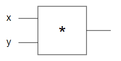
The circuit takes two real-valued inputs x and y and computes x * y with the * gate. Javascript version of this would very simply look something like this:

var forwardMultiplyGate = function(x, y) {
  return x * y;
};
forwardMultiplyGate(-2, 3); // returns -6. Exciting.

And in math form we can think of this gate as implementing the real-valued function:

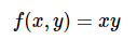
As with this example, all of our gates will take one or two inputs and produce a single output value.

The Goal

The problem we are interested in studying looks as follows:

1. We provide a given circuit some specific input values (e.g. x = -2, y = 3)
2. The circuit computes an output value (e.g. -6)
3. The core question then becomes: How should one tweak the input slightly to increase the output?

In this case, in what direction should we change x,y to get a number larger than -6? Note that, for example, x = -1.99 and y = 2.99 gives x * y = -5.95, which is higher than -6.0. Don’t get confused by this: -5.95 is better (higher) than -6.0. It’s an improvement of 0.05, even though the magnitude of -5.95 (the distance from zero) happens to be lower.

Strategy #1: Random Local Search

Okay. So wait, we have a circuit, we have some inputs and we just want to tweak them slightly to increase the output value? Why is this hard? We can easily “forward” the circuit to compute the output for any given x and y. So isn’t this trivial? Why don’t we tweak x and y randomly and keep track of the tweak that works best:

// circuit with single gate for now
var forwardMultiplyGate = function(x, y) { return x * y; };
var x = -2, y = 3; // some input values

// try changing x,y randomly small amounts and keep track of what works best
var tweak_amount = 0.01;
var best_out = -Infinity;
var best_x = x, best_y = y;
for(var k = 0; k < 100; k++) {
  var x_try = x + tweak_amount * (Math.random() * 2 - 1); // tweak x a bit
  var y_try = y + tweak_amount * (Math.random() * 2 - 1); // tweak y a bit
  var out = forwardMultiplyGate(x_try, y_try);
  if(out > best_out) {
    // best improvement yet! Keep track of the x and y
    best_out = out; 
    best_x = x_try, best_y = y_try;
  }
}

When I run this, I get best_x = -1.9928, best_y = 2.9901, and best_out = -5.9588. Again, -5.9588 is higher than -6.0. So, we’re done, right? Not quite: This is a perfectly fine strategy for tiny problems with a few gates if you can afford the compute time, but it won’t do if we want to eventually consider huge circuits with millions of inputs. It turns out that we can do much better.

Stategy #2: Numerical Gradient

Here’s a better way. Remember again that in our setup we are given a circuit (e.g. our circuit with a single * gate) and some particular input (e.g. x = -2, y = 3). The gate computes the output (-6) and now we’d like to tweak x and y to make the output higher.

A nice intuition for what we’re about to do is as follows: Imagine taking the output value that comes out from the circuit and tugging on it in the positive direction. This positive tension will in turn translate through the gate and induce forces on the inputs x and y. Forces that tell us how x and y should change to increase the output value.

What might those forces look like in our specific example? Thinking through it, we can intuit that the force on x should also be positive, because making x slightly larger improves the circuit’s output. For example, increasing x from x = -2 to x = -1 would give us output -3 - much larger than -6. On the other hand, we’d expect a negative force induced on y that pushes it to become lower (since a lower y, such as y = 2, down from the original y = 3 would make output higher: 2 x -2 = -4, again, larger than -6). That’s the intuition to keep in mind, anyway. As we go through this, it will turn out that forces I’m describing will in fact turn out to be the derivative of the output value with respect to its inputs (x and y). You may have heard this term before.

The derivative can be thought of as a force on each input as we pull on the output to become higher.

So how do we exactly evaluate this force (derivative)? It turns out that there is a very simple procedure for this. We will work backwards: Instead of pulling on the circuit’s output, we’ll iterate over every input one by one, increase it very slightly and look at what happens to the output value. The amount the output changes in response is the derivative. Enough intuitions for now. Lets look at the mathematical definition. We can write down the derivative for our function with respect to the inputs. For example, the derivative with respect to x can be computed as:

∂f(x,y)∂x=f(x+h,y)−f(x,y)h∂f(x,y)∂x=f(x+h,y)−f(x,y)h

Where hh is small - it’s the tweak amount. Also, if you’re not very familiar with calculus it is important to note that in the left-hand side of the equation above, the horizontal line does not indicate division. The entire symbol ∂f(x,y)∂x∂f(x,y)∂x is a single thing: the derivative of the function f(x,y)f(x,y) with respect to xx. The horizontal line on the right is division. I know it’s confusing but it’s standard notation. Anyway, I hope it doesn’t look too scary because it isn’t: The circuit was giving some initial output f(x,y)f(x,y), and then we changed one of the inputs by a tiny amount hh and read the new output f(x+h,y)f(x+h,y). Subtracting those two quantities tells us the change, and the division by hh just normalizes this change by the (arbitrary) tweak amount we used. In other words it’s expressing exactly what I described above and translates directly to this code:

var x = -2, y = 3;
var out = forwardMultiplyGate(x, y); // -6
var h = 0.0001;

// compute derivative with respect to x
var xph = x + h; // -1.9999
var out2 = forwardMultiplyGate(xph, y); // -5.9997
var x_derivative = (out2 - out) / h; // 3.0

// compute derivative with respect to y
var yph = y + h; // 3.0001
var out3 = forwardMultiplyGate(x, yph); // -6.0002
var y_derivative = (out3 - out) / h; // -2.0

Lets walk through x for example. We turned the knob from x to x + h and the circuit responded by giving a higher value (note again that yes, -5.9997 is higher than -6: -5.9997 > -6). The division by h is there to normalize the circuit’s response by the (arbitrary) value of h we chose to use here. Technically, you want the value of h to be infinitesimal (the precise mathematical definition of the gradient is defined as the limit of the expression as h goes to zero), but in practice h=0.00001 or so works fine in most cases to get a good approximation. Now, we see that the derivative w.r.t. x is +3. I’m making the positive sign explicit, because it indicates that the circuit is tugging on x to become higher. The actual value, 3 can be interpreted as the force of that tug.

The derivative with respect to some input can be computed by tweaking that input by a small amount and observing the change on the output value.

By the way, we usually talk about the derivative with respect to a single input, or about a gradient with respect to all the inputs. The gradient is just made up of the derivatives of all the inputs concatenated in a vector (i.e. a list). Crucially, notice that if we let the inputs respond to the tug by following the gradient a tiny amount (i.e. we just add the derivative on top of every input), we can see that the value increases, as expected:

var step_size = 0.01;
var out = forwardMultiplyGate(x, y); // before: -6
x = x + step_size * x_derivative; // x becomes -1.97
y = y + step_size * y_derivative; // y becomes 2.98
var out_new = forwardMultiplyGate(x, y); // -5.87! exciting.

As expected, we changed the inputs by the gradient and the circuit now gives a slightly higher value (-5.87 > -6.0). That was much simpler than trying random changes to x and y, right? A fact to appreciate here is that if you take calculus you can prove that the gradient is, in fact, the direction of the steepest increase of the function. There is no need to monkey around trying out random pertubations as done in Strategy #1. Evaluating the gradient requires just three evaluations of the forward pass of our circuit instead of hundreds, and gives the best tug you can hope for (locally) if you are interested in increasing the value of the output.

Bigger step is not always better. Let me clarify on this point a bit. It is important to note that in this very simple example, using a bigger step_size than 0.01 will always work better. For example, step_size = 1.0 gives output -1 (higer, better!), and indeed infinite step size would give infinitely good results. The crucial thing to realize is that once our circuits get much more complex (e.g. entire neural networks), the function from inputs to the output value will be more chaotic and wiggly. The gradient guarantees that if you have a very small (indeed, infinitesimally small) step size, then you will definitely get a higher number when you follow its direction, and for that infinitesimally small step size there is no other direction that would have worked better. But if you use a bigger step size (e.g. step_size = 0.01) all bets are off. The reason we can get away with a larger step size than infinitesimally small is that our functions are usually relatively smooth. But really, we’re crossing our fingers and hoping for the best.

Hill-climbing analogy. One analogy I’ve heard before is that the output value of our circut is like the height of a hill, and we are blindfolded and trying to climb upwards. We can sense the steepness of the hill at our feet (the gradient), so when we shuffle our feet a bit we will go upwards. But if we took a big, overconfident step, we could have stepped right into a hole.

Great, I hope I’ve convinced you that the numerical gradient is indeed a very useful thing to evaluate, and that it is cheap. But. It turns out that we can do even better.

Strategy #3: Analytic Gradient

In the previous section we evaluated the gradient by probing the circuit’s output value, independently for every input. This procedure gives you what we call a numerical gradient. This approach, however, is still expensive because we need to compute the circuit’s output as we tweak every input value independently a small amount. So the complexity of evaluating the gradient is linear in number of inputs. But in practice we will have hundreds, thousands or (for neural networks) even tens to hundreds of millions of inputs, and the circuits aren’t just one multiply gate but huge expressions that can be expensive to compute. We need something better.

Luckily, there is an easier and much faster way to compute the gradient: we can use calculus to derive a direct expression for it that will be as simple to evaluate as the circuit’s output value. We call this an analytic gradient and there will be no need for tweaking anything. You may have seen other people who teach Neural Networks derive the gradient in huge and, frankly, scary and confusing mathematical equations (if you’re not well-versed in maths). But it’s unnecessary. I’ve written plenty of Neural Nets code and I rarely have to do mathematical derivation longer than two lines, and 95% of the time it can be done without writing anything at all. That is because we will only ever derive the gradient for very small and simple expressions (think of it as the base case) and then I will show you how we can compose these very simply with chain rule to evaluate the full gradient (think inductive/recursive case).

The analytic derivative requires no tweaking of the inputs. It can be derived using mathematics (calculus).

If you remember your product rules, power rules, quotient rules, etc. (see e.g. derivative rules or wiki page), it’s very easy to write down the derivitative with respect to both x and y for a small expression such as x * y. But suppose you don’t remember your calculus rules. We can go back to the definition. For example, here’s the expression for the derivative w.r.t x:

∂f(x,y)∂x=f(x+h,y)−f(x,y)h∂f(x,y)∂x=f(x+h,y)−f(x,y)h

(Technically I’m not writing the limit as h goes to zero, forgive me math people). Okay and lets plug in our function ( f(x,y)=xyf(x,y)=xy ) into the expression. Ready for the hardest piece of math of this entire article? Here we go:

∂f(x,y)∂x=f(x+h,y)−f(x,y)h=(x+h)y−xyh=xy+hy−xyh=hyh=y∂f(x,y)∂x=f(x+h,y)−f(x,y)h=(x+h)y−xyh=xy+hy−xyh=hyh=y

That’s interesting. The derivative with respect to x is just equal to y. Did you notice the coincidence in the previous section? We tweaked x to x+h and calculated x_derivative = 3.0, which exactly happens to be the value of y in that example. It turns out that wasn’t a coincidence at all because that’s just what the analytic gradient tells us the x derivative should be for f(x,y) = x * y. The derivative with respect to y, by the way, turns out to be x, unsurprisingly by symmetry. So there is no need for any tweaking! We invoked powerful mathematics and can now transform our derivative calculation into the following code:

var x = -2, y = 3;
var out = forwardMultiplyGate(x, y); // before: -6
var x_gradient = y; // by our complex mathematical derivation above
var y_gradient = x;

var step_size = 0.01;
x += step_size * x_gradient; // -1.97
y += step_size * y_gradient; // 2.98
var out_new = forwardMultiplyGate(x, y); // -5.87. Higher output! Nice.

To compute the gradient we went from forwarding the circuit hundreds of times (Strategy #1) to forwarding it only on order of number of times twice the number of inputs (Strategy #2), to forwarding it a single time! And it gets EVEN better, since the more expensive strategies (#1 and #2) only give an approximation of the gradient, while #3 (the fastest one by far) gives you the exact gradient. No approximations. The only downside is that you should be comfortable with some calculus 101.

Lets recap what we have learned:

• INPUT: We are given a circuit, some inputs and compute an output value.
• OUTPUT: We are then interested finding small changes to each input (independently) that would make the output higher.
• Strategy #1: One silly way is to randomly search for small pertubations of the inputs and keep track of what gives the highest increase in output.
• Strategy #2: We saw we can do much better by computing the gradient. Regardless of how complicated the circuit is, the numerical gradient is very simple (but relatively expensive) to compute. We compute it by probing the circuit’s output value as we tweak the inputs one at a time.
• Strategy #3: In the end, we saw that we can be even more clever and analytically derive a direct expression to get the analytic gradient. It is identical to the numerical gradient, it is fastest by far, and there is no need for any tweaking.

In practice by the way (and we will get to this once again later), all Neural Network libraries always compute the analytic gradient, but the correctness of the implementation is verified by comparing it to the numerical gradient. That’s because the numerical gradient is very easy to evaluate (but can be a bit expensive to compute), while the analytic gradient can contain bugs at times, but is usually extremely efficient to compute. As we will see, evaluating the gradient (i.e. while doing backprop, or backward pass) will turn out to cost about as much as evaluating the forward pass.

next:  https://www.cnblogs.com/zhangzhiwei122/p/15887335.html