PySpark - Performance Tuning with Apache Spark

 

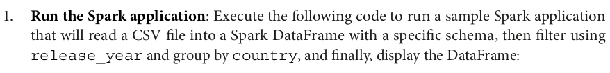
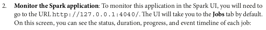
from pyspark.sql import SparkSession

# Create a new SparkSession
spark = (SparkSession
         .builder
         .appName("monitor-spark-ui")
         .master("spark://ZZHPC:7077")
         .config("spark.executor.memory", "512m")
         .getOrCreate())

# Set log level to ERROR
spark.sparkContext.setLogLevel("ERROR")

from pyspark.sql.types import StructType, StructField, StringType, IntegerType, DateType

# Define a Schema
schema = StructType([
    StructField("show_id", StringType(), True),
    StructField("type", StringType(), True),
    StructField("title", StringType(), True),
    StructField("director", StringType(), True),
    StructField("cast", StringType(), True),
    StructField("country", StringType(), True),
    StructField("date_added", DateType(), True),
    StructField("release_year", IntegerType(), True),
    StructField("rating", StringType(), True),
    StructField("duration", StringType(), True),
    StructField("listed_in", StringType(), True),
    StructField("description", StringType(), True)])

# Read CSV file into a DataFrame
df = (spark.read.format("csv")
      .option("header", "true")
      .schema(schema)
      .load("../data/netflix_titles.csv"))

# Filter rows where release_year ge is greater than 2020
df = df.filter(df.release_year > 2020)

# Group by country and count
df = df.groupBy("country").count()

# Show the result
df.show()

 

 

 

 

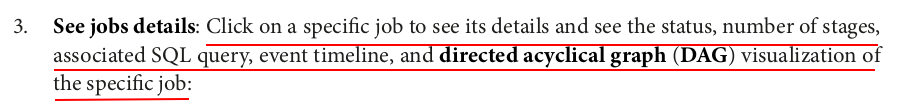
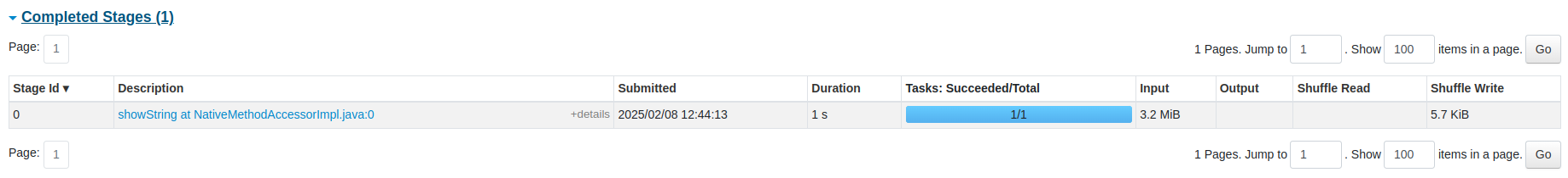
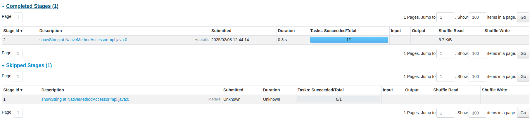
You can also see the list of stages grouped by state (active, pending, completed, skipped, or failed):

 

 

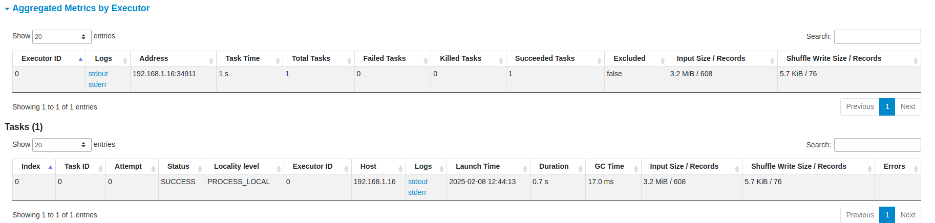
You can also see the status, executor ID, host, index, attempt, launch time, duration, input/output/shuffle metrics, and error message (if any) of the task.

 

 

 

 

 

 

spark.stop()

 

from pyspark.sql import SparkSession 
from pyspark.sql.functions import rand, when, pandas_udf, PandasUDFType
from pyspark.sql.types import BooleanType
import pandas as pd

spark = (SparkSession
         .builder
         .appName("broadcast-variables")
         .master("spark://ZZHPC:7077")
         .config("spark.executor.memory", "512m")
         .getOrCreate())

spark.sparkContext.setLogLevel("ERROR")

 

large_df = (spark.range(0, 1000000)
            .withColumn("salary", 100 * (rand() * 100).cast("int"))
            .withColumn("gender", when((rand() * 2).cast("int") == 0, "M").otherwise("F"))
            .withColumn("country_code", 
                        when((rand() * 4).cast("int") == 0, "US")
                        .when((rand() * 4).cast("int") == 1, "CN")
                        .when((rand() * 4).cast("int") == 2, "IN")
                        .when((rand() * 4).cast("int") == 3, "BR")))
large_df.show(5)

 

+---+------+------+------------+
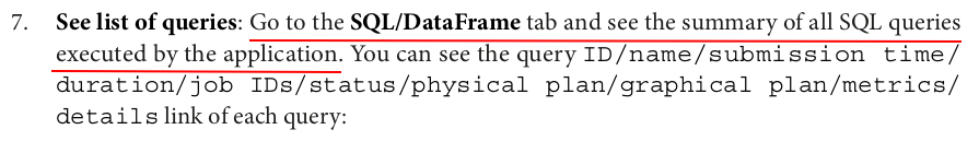
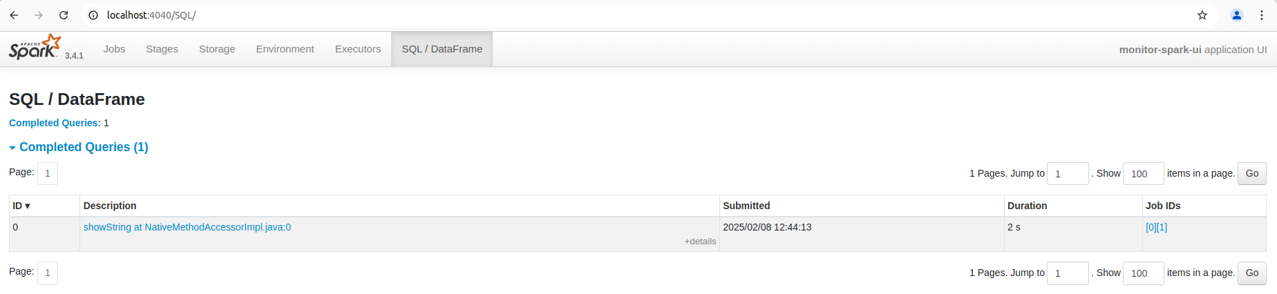
| id|salary|gender|country_code|
+---+------+------+------------+
|  0|  2200|     F|          BR|
|  1|   800|     F|          BR|
|  2|  4900|     M|          IN|
|  3|  5600|     M|        null|
|  4|  4300|     M|          US|
+---+------+------+------------+
only showing top 5 rows

 

The spark.range() function in Apache Spark is used to create a DataFrame containing a range of values, typically used when you need a simple DataFrame with numbers. This function is often used for creating a range of integers that can then be manipulated or transformed in subsequent operations.

spark.range(start, end=None, step=1, numPartitions=None)

Parameters:

1. start:

   • The start value of the range (inclusive).
   • This parameter is required.

2. end (optional):

   • The end value of the range (exclusive).
   • If end is not specified, start is interpreted as end and start becomes 0.

3. step (optional):

   • The step size between consecutive values in the range. The default value is 1.
   • For example, if you want a range of even numbers, you could set step=2.

4. numPartitions (optional):

   • Specifies the number of partitions in the resulting DataFrame.
   • If not specified, the number of partitions is automatically chosen based on the number of rows in the DataFrame.

df = spark.range(10)
df.show()

 

+---+
| id|
+---+
|  0|
|  1|
|  2|
|  3|
|  4|
|  5|
|  6|
|  7|
|  8|
|  9|
+---+

While spark.range() by default creates a DataFrame with a column named id, you can use the toDF() method to rename the column(s). Here's how you can do it:

Customizing the Column Name:

df = spark.range(5, 15).toDF("my_custom_column_name")
df.show()

 

+-------------------+
|my_custom_column_name|
+-------------------+
|                  5|
|                  6|
|                  7|
|                  8|
|                  9|
|                 10|
|                 11|
|                 12|
|                 13|
|                 14|
+-------------------+

 

# Define lookup table
lookup = {"US": "United States", "CN": "China", "IN": "India", "BR": "Brazil", "RU": "Russia"}

# Create broadcast variable
broadcast_lookup = spark.sparkContext.broadcast(lookup)

The broadcast() function is used to efficiently share a read-only variable (like the lookup dictionary) across all workers in the cluster. This ensures that each worker node can access the dictionary without duplicating the data.

 

@pandas_udf('string', PandasUDFType.SCALAR)
def country_convert(s):
    return s.map(broadcast_lookup.value)

• @pandas_udf('string'): This decorator turns the country_convert function into a pandas UDF. The 'string' argument indicates that the UDF will return a column of strings.
• PandasUDFType.SCALAR: This specifies that the UDF operates element-wise on the input, similar to a regular Python function applied to each row in a pandas Series.

 

• s.map() is a method specific to pandas Series. It applies a function or a mapping to each element in the Series (column of a DataFrame). 
• broadcast_lookup.value: Since broadcast_lookup is a broadcast variable, broadcast_lookup.value gives access to the original lookup dictionary.

 

large_df.withColumn("country_name", country_convert(large_df.country_code)).show(5)

 

+---+------+------+------------+-------------+
| id|salary|gender|country_code| country_name|
+---+------+------+------------+-------------+
|  0|  2200|     F|          BR|       Brazil|
|  1|   800|     F|          BR|       Brazil|
|  2|  4900|     M|          IN|        India|
|  3|  5600|     M|        null|         null|
|  4|  4300|     M|          US|United States|
+---+------+------+------------+-------------+
only showing top 5 rows

 

@pandas_udf(BooleanType(), PandasUDFType.SCALAR)
def filter_unknown_country(s):
    return s.isin(broadcast_lookup.value)

 

large_df.filter(filter_unknown_country(large_df.country_code)).show(5)

 

+---+------+------+------------+
| id|salary|gender|country_code|
+---+------+------+------------+
|  0|  2200|     F|          BR|
|  1|   800|     F|          BR|
|  2|  4900|     M|          IN|
|  4|  4300|     M|          US|
|  6|  7500|     M|          BR|
+---+------+------+------------+
only showing top 5 rows

 

spark.stop()

 

from pyspark.sql import SparkSession 
from pyspark.sql.functions import col, avg, date_sub, current_date, rand, when, broadcast

spark = (SparkSession
         .builder
         .appName("optimize-data-shuffles")
         .master("spark://ZZHPC:7077")
         .getOrCreate())

spark.sparkContext.setLogLevel("ERROR")

 

large_df = (spark.range(0, 1000000)
            .withColumn("date", date_sub(current_date(), (rand() * 365).cast("int")))
            .withColumn("age", (rand() * 100).cast("int"))
            .withColumn("salary", 100*(rand() * 100).cast("int"))
            .withColumn("gender", when((rand() * 2).cast("int") == 0, "M").otherwise("F"))
            .withColumn("grade", 
                        when((rand() * 5).cast("int") == 0, "IC")
                        .when((rand() * 5).cast("int") == 1, "IC-2")
                        .when((rand() * 5).cast("int") == 2, "M1")
                        .when((rand() * 5).cast("int") == 3, "M2")
                        .when((rand() * 5).cast("int") == 4, "IC-3")
                        .otherwise("M3")))
large_df.show(5)

 

+---+----------+---+------+------+-----+
| id|      date|age|salary|gender|grade|
+---+----------+---+------+------+-----+
|  0|2024-12-25| 87|  4900|     F| IC-2|
|  1|2024-11-05| 55|   400|     M| IC-3|
|  2|2024-04-23| 62|  7600|     F|   M3|
|  3|2024-06-22| 36|  3500|     M|   M3|
|  4|2024-07-23| 45|  7000|     M|   IC|
+---+----------+---+------+------+-----+
only showing top 5 rows

 

# Filter the DataFrame by age
df_filtered = large_df.filter(col("age") >= 55)

# Map the DataFrame by adding 10% bonus to salary
df_mapped = df_filtered.withColumn("bonus", col("salary") * 1.1)

# Locally aggregate the DataFrame by computing the average bonus by age
df_aggregated = df_mapped.groupBy("age").agg(avg("bonus"))
df_aggregated = df_mapped.groupBy("age").avg("bonus")
# These two ways of writing got the same results and execution plans.

# Print the result
df_aggregated.show(5)

 

+---+-----------------+
|age|       avg(bonus)|
+---+-----------------+
| 85|5390.456570155902|
| 65|5428.148558758315|
| 78|5350.175996818137|
| 81|5430.669947770189|
| 76|5429.570160566471|
+---+-----------------+
only showing top 5 rows

 

df_aggregated.explain()

 

== Physical Plan ==
AdaptiveSparkPlan isFinalPlan=false
+- HashAggregate(keys=[age#5], functions=[avg(bonus#52)])
   +- Exchange hashpartitioning(age#5, 200), ENSURE_REQUIREMENTS, [plan_id=123]
      +- HashAggregate(keys=[age#5], functions=[partial_avg(bonus#52)])
         +- Project [age#5, (cast(salary#9 as double) * 1.1) AS bonus#52]
            +- Filter (isnotnull(age#5) AND (age#5 >= 55))
               +- Project [age#5, (cast((rand(5924895267823410885) * 100.0) as int) * 100) AS salary#9]
                  +- Project [cast((rand(-908904385464407571) * 100.0) as int) AS age#5]
                     +- Range (0, 1000000, step=1, splits=6)

 

What is the difference between "partial_avg(bonus#52)" and "avg(bonus#52)" in above execution plan?

1. partial_avg(bonus#52):

• This represents a partial aggregation that is performed locally on each partition before the data is shuffled across the cluster.
• Partial Aggregation: In Spark, when performing an aggregation like avg(), the process can be split into two steps:
  • Partial Aggregation: Each partition computes a partial result, e.g., a sum and count of the bonus values within that partition.
  • Final Aggregation: After partial results are computed, Spark will then combine them from all partitions (this is the global aggregation step).

     In this case, partial_avg(bonus#52) is the partial computation of the average bonus value done locally on each partition. It calculates the sum and count of bonus for each partition independently.

• Purpose: This step is designed to minimize the amount of data that needs to be shuffled across the cluster. By performing partial aggregation within each partition, Spark reduces the size of the data that will be shuffled.

2. avg(bonus#52):

• This represents the final aggregation step where Spark combines the partial results from all the partitions to compute the final average for each age group across the entire dataset.
• After the partial aggregation (partial_avg), Spark needs to aggregate the results from different worker nodes and calculate the global average, which is represented by avg(bonus#52) in the plan.
• This final step involves combining the partial sums and counts from all the partitions to compute the overall average of the bonus.

Why Two Stages for Aggregation?

Spark uses a two-phase aggregation strategy to improve performance:

1. Partial Aggregation (Before Shuffling):

   • In the first phase (partial_avg(bonus#52)), Spark computes partial sums and counts for each group (in this case, age) within each partition. This reduces the amount of data that needs to be shuffled, as only the partial results are exchanged between nodes.

2. Global Aggregation (After Shuffling):

   • In the second phase (avg(bonus#52)), Spark takes the partial results from each partition and combines them to compute the final result. The partial sums and counts are aggregated across all partitions to produce the final average.

Why Is This Optimization Important?

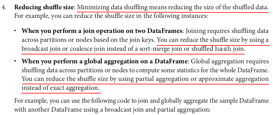
• Reduced Shuffle Size: By aggregating locally on each partition before shuffling the data, Spark significantly reduces the amount of data that needs to be transferred between nodes. Instead of sending all the individual bonus values across the network, Spark only needs to send the partial sums and counts for each group, which is much smaller in size.

• Performance: The two-phase aggregation minimizes network overhead and speeds up the overall computation, especially when dealing with large datasets.

 

# Create another DataFrame with some dummy data
df2 = spark.createDataFrame([(25, "A"), (30, "B"), (35, "C"), (40, "D"), (45, "E"), (50, "F"), (55, "G"), (60, "H"), (65, "I"), (70, "J")], ["age", "level"])

# Join the two DataFrames by age using broadcast join
df_joined = large_df.join(broadcast(df2), "age")

# Globally aggregate the joined DataFrame by computing the sum of salary by level using partial aggregation
df_aggregated = df_joined.groupBy("level").avg("salary")

# Print the result
df_aggregated.show()

 

+-----+------------------+
|level|       avg(salary)|
+-----+------------------+
|    F|  4927.46020622685|
|    E| 4943.687072090213|
|    B| 4969.149781485896|
|    D| 4915.887096774193|
|    C| 4926.426148627814|
|    J| 4941.961219955565|
|    A| 5030.829199149539|
|    G| 4943.469143199521|
|    I|4934.6805079621045|
|    H| 4861.916120055655|
+-----+------------------+

 

df_aggregated.explain()

 

== Physical Plan ==
AdaptiveSparkPlan isFinalPlan=false
+- HashAggregate(keys=[level#162], functions=[avg(salary#9)])
   +- Exchange hashpartitioning(level#162, 200), ENSURE_REQUIREMENTS, [plan_id=554]
      +- HashAggregate(keys=[level#162], functions=[partial_avg(salary#9)])
         +- Project [salary#9, level#162]
            +- BroadcastHashJoin [cast(age#5 as bigint)], [age#161L], Inner, BuildRight, false
               :- Filter isnotnull(age#5)
               :  +- Project [age#5, (cast((rand(5924895267823410885) * 100.0) as int) * 100) AS salary#9]
               :     +- Project [cast((rand(-908904385464407571) * 100.0) as int) AS age#5]
               :        +- Range (0, 1000000, step=1, splits=6)
               +- BroadcastExchange HashedRelationBroadcastMode(List(input[0, bigint, false]),false), [plan_id=549]
                  +- Filter isnotnull(age#161L)
                     +- Scan ExistingRDD[age#161L,level#162]

 

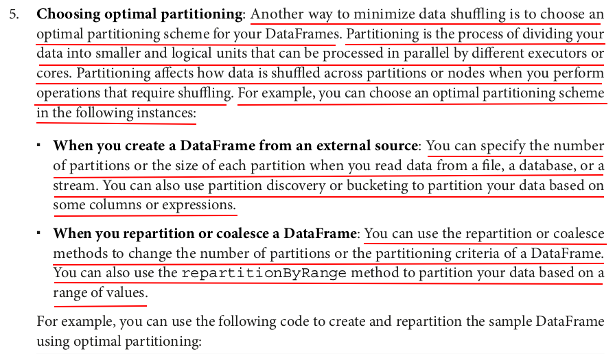
# Repartition the DataFrame by gender with 2 partitions
df_repartitioned = large_df.repartition(col("gender"))

# Repartition the DataFrame by age range with 5 partitions
df_repartitioned_by_range = large_df.repartitionByRange(5, col("age"))

 

 

large_df.explain()

 

== Physical Plan ==
*(1) Project [id#0L, date#2, age#5, salary#9, gender#14, CASE WHEN (cast((rand(-1974792337886645978) * 5.0) as int) = 0) THEN IC WHEN (cast((rand(-7500129802891786044) * 5.0) as int) = 1) THEN IC-2 WHEN (cast((rand(4189861129437882142) * 5.0) as int) = 2) THEN M1 WHEN (cast((rand(8546001166606760019) * 5.0) as int) = 3) THEN M2 WHEN (cast((rand(3666749250523696306) * 5.0) as int) = 4) THEN IC-3 ELSE M3 END AS grade#20]
+- *(1) Project [id#0L, date#2, age#5, salary#9, CASE WHEN (cast((rand(4010303950217595915) * 2.0) as int) = 0) THEN M ELSE F END AS gender#14]
   +- *(1) Project [id#0L, date#2, age#5, (cast((rand(5924895267823410885) * 100.0) as int) * 100) AS salary#9]
      +- *(1) Project [id#0L, date#2, cast((rand(-908904385464407571) * 100.0) as int) AS age#5]
         +- *(1) Project [id#0L, date_sub(2025-02-08, cast((rand(2550221140511847604) * 365.0) as int)) AS date#2]
            +- *(1) Range (0, 1000000, step=1, splits=6)

 

df_repartitioned.explain()

 

== Physical Plan ==
AdaptiveSparkPlan isFinalPlan=false
+- Exchange hashpartitioning(gender#14, 200), REPARTITION_BY_COL, [plan_id=606]
   +- Project [id#0L, date#2, age#5, salary#9, gender#14, CASE WHEN (cast((rand(-1974792337886645978) * 5.0) as int) = 0) THEN IC WHEN (cast((rand(-7500129802891786044) * 5.0) as int) = 1) THEN IC-2 WHEN (cast((rand(4189861129437882142) * 5.0) as int) = 2) THEN M1 WHEN (cast((rand(8546001166606760019) * 5.0) as int) = 3) THEN M2 WHEN (cast((rand(3666749250523696306) * 5.0) as int) = 4) THEN IC-3 ELSE M3 END AS grade#20]
      +- Project [id#0L, date#2, age#5, salary#9, CASE WHEN (cast((rand(4010303950217595915) * 2.0) as int) = 0) THEN M ELSE F END AS gender#14]
         +- Project [id#0L, date#2, age#5, (cast((rand(5924895267823410885) * 100.0) as int) * 100) AS salary#9]
            +- Project [id#0L, date#2, cast((rand(-908904385464407571) * 100.0) as int) AS age#5]
               +- Project [id#0L, date_sub(2025-02-08, cast((rand(2550221140511847604) * 365.0) as int)) AS date#2]
                  +- Range (0, 1000000, step=1, splits=6)

 

df_repartitioned_by_range.explain()

 

== Physical Plan ==
AdaptiveSparkPlan isFinalPlan=false
+- Exchange rangepartitioning(age#5 ASC NULLS FIRST, 5), REPARTITION_BY_NUM, [plan_id=634]
   +- Project [id#0L, date#2, age#5, salary#9, gender#14, CASE WHEN (cast((rand(-1974792337886645978) * 5.0) as int) = 0) THEN IC WHEN (cast((rand(-7500129802891786044) * 5.0) as int) = 1) THEN IC-2 WHEN (cast((rand(4189861129437882142) * 5.0) as int) = 2) THEN M1 WHEN (cast((rand(8546001166606760019) * 5.0) as int) = 3) THEN M2 WHEN (cast((rand(3666749250523696306) * 5.0) as int) = 4) THEN IC-3 ELSE M3 END AS grade#20]
      +- Project [id#0L, date#2, age#5, salary#9, CASE WHEN (cast((rand(4010303950217595915) * 2.0) as int) = 0) THEN M ELSE F END AS gender#14]
         +- Project [id#0L, date#2, age#5, (cast((rand(5924895267823410885) * 100.0) as int) * 100) AS salary#9]
            +- Project [id#0L, date#2, cast((rand(-908904385464407571) * 100.0) as int) AS age#5]
               +- Project [id#0L, date_sub(2025-02-08, cast((rand(2550221140511847604) * 365.0) as int)) AS date#2]
                  +- Range (0, 1000000, step=1, splits=6)

 

num_partitions = large_df.rdd.getNumPartitions()
print(f"Number of partitions: {num_partitions}")

# Number of partitions: 6


num_partitions = df_repartitioned.rdd.getNumPartitions()
print(f"Number of partitions: {num_partitions}")

# Number of partitions: 2


num_partitions = df_repartitioned_by_range.rdd.getNumPartitions()
print(f"Number of partitions: {num_partitions}")

# Number of partitions: 5

 

 

spark.stop()

 

from pyspark.sql import SparkSession 
from pyspark.sql.functions import rand, col, when, broadcast, concat, lit

spark = (SparkSession
         .builder
         .appName("avoid-data-skew")
         .master("spark://ZZHPC:7077")
         .getOrCreate())

spark.sparkContext.setLogLevel("ERROR")

 

import time

def measure_time(query):
    start = time.time()
    query.collect() # Force the query execution by calling an action
    end = time.time()
    print(f"Execution time: {end - start} seconds")

 

# A large data frame with 10 million rows and two columns: id and value
large_df = spark.range(0, 10000000).withColumn("value", rand(seed=42))

# A skewed data frame with 1 million rows and two columns: id and value
skewed_df = spark.range(0, 1000000).withColumn("value", rand(seed=42)).withColumn("id", when(col("id") % 4 == 0, 0).otherwise(col("id")))

 

large_df.rdd.getNumPartitions()

# 6

skewed_df.rdd.getNumPartitions()

# 6

 

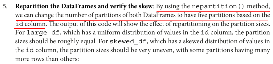
large_df_repartitioned = large_df.repartition(5, "id")
num_partitions = large_df_repartitioned.rdd.getNumPartitions()
print(f"Number of partitions: {num_partitions}")

partition_sizes = large_df_repartitioned.rdd.glom().map(len).collect()
print(f"Partition sizes: {partition_sizes}")

skewed_df_repartitioned = skewed_df.repartition(5, "id")
num_partitions = skewed_df_repartitioned.rdd.getNumPartitions()
print(f"Number of partitions: {num_partitions}")

partition_sizes = skewed_df_repartitioned.rdd.glom().map(len).collect()
print(f"Partition sizes: {partition_sizes}")

 

Number of partitions: 5
Partition sizes: [1998962, 2000902, 1999898, 2000588, 1999650]
Number of partitions: 5
Partition sizes: [400054, 150144, 149846, 149903, 150053]

 

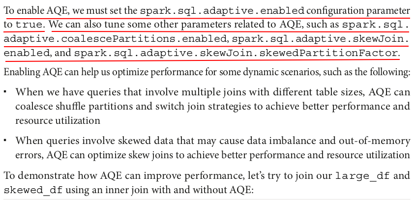
spark.conf.set("spark.sql.adaptive.enabled", "false")

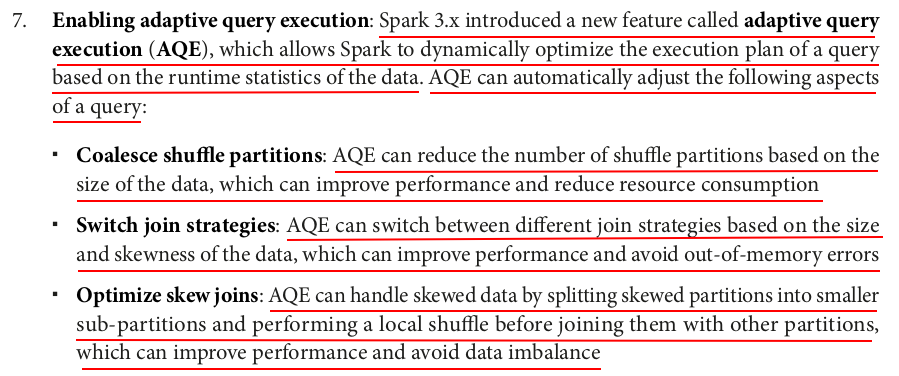
What is Adaptive Query Execution (AQE)?

• Adaptive Query Execution (AQE) is a feature introduced in Spark 3.0 that allows Spark to optimize query execution dynamically, based on runtime statistics and data distribution. It enables Spark to make adaptive decisions during query execution, such as:
  • Dynamic Partition Pruning: Spark can dynamically prune partitions during the execution of a query based on actual data.
  • Join Strategy Selection: Spark can choose the best join strategy (broadcast join, shuffle join, etc.) at runtime based on data sizes.
  • Coalescing Shuffle Partitions: Spark can merge small shuffle partitions at runtime to reduce the number of tasks, improving efficiency.

AQE helps improve the performance of queries, especially those with skewed data or complex joins, by making runtime adjustments based on actual data statistics.

What Happens When You Set "spark.sql.adaptive.enabled" to "false"?

• Disabling AQE: Setting "spark.sql.adaptive.enabled" to "false" turns off Adaptive Query Execution. This means that Spark will not apply any of the AQE optimizations during query execution.

• Without AQE, Spark will rely on static query plans that were created at the start of query execution. This means that:

  • Spark will not dynamically adjust partition sizes or pruning during query execution.
  • Spark will not change join strategies based on data distribution.
  • Spark will not merge small shuffle partitions to improve efficiency.

Why Would You Disable AQE?

While AQE can significantly improve query performance in many scenarios, there might be cases where you want to disable it:

1. Performance Issues: In some rare cases, AQE might introduce overhead or cause performance degradation if the runtime optimizations are not suitable for your workload. Disabling AQE can help in such cases.

2. Debugging and Reproducibility: Disabling AQE ensures that the query execution plan is static and does not change dynamically based on data. This can help with debugging and understanding exactly how Spark will execute a query.

3. Specific Optimizations: Some users may prefer to control query optimizations manually and not rely on Spark's dynamic decisions.

 

spark.conf.set("spark.sql.autoBroadcastJoinThreshold", -1)

What Does It Do?

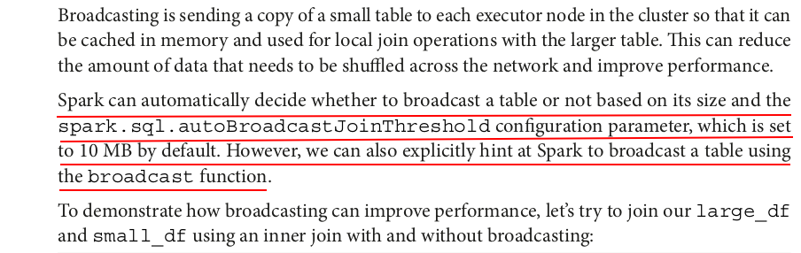
• spark.sql.autoBroadcastJoinThreshold: This parameter controls the size of the smaller DataFrame that will be automatically broadcast to all worker nodes during a join operation. If the size of the smaller DataFrame exceeds the specified threshold, Spark will not use a broadcast join. Conversely, if the size is below the threshold, Spark will automatically broadcast the smaller DataFrame to all worker nodes to improve the performance of the join operation.

  • Default Value: By default, this threshold is set to 10MB (10 * 1024 * 1024 bytes), meaning that if the smaller DataFrame is less than 10MB, it will be broadcasted automatically during a join.

Setting the Threshold to -1:

• By setting the spark.sql.autoBroadcastJoinThreshold to -1, you're effectively disabling automatic broadcast joins altogether.

  • Why -1?: When the threshold is set to -1, Spark will never automatically broadcast any DataFrame, regardless of its size. Even if the DataFrame is small enough to be broadcasted, Spark will not attempt to do so. This could be useful if you want more control over whether or not broadcast joins are used in your queries, or if you're seeing performance issues related to broadcast joins and want to disable them entirely.

 

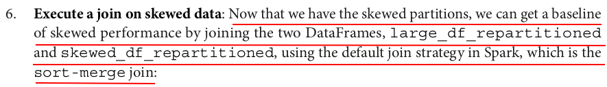
# Join the non-skewed DataFrames using the default join strategy (sort-merge join)
inner_join_df = large_df_repartitioned.join(skewed_df_repartitioned, "id")
measure_time(inner_join_df)

 

Execution time: 8.1443510055542 seconds

 

inner_join_df.explain()

 

== Physical Plan ==
*(5) Project [id#0L, value#2, value#7]
+- *(5) SortMergeJoin [id#0L], [id#10L], Inner
   :- *(2) Sort [id#0L ASC NULLS FIRST], false, 0
   :  +- Exchange hashpartitioning(id#0L, 200), REPARTITION_BY_NUM, [plan_id=133]
   :     +- *(1) Project [id#0L, rand(42) AS value#2]
   :        +- *(1) Range (0, 10000000, step=1, splits=6)
   +- *(4) Sort [id#10L ASC NULLS FIRST], false, 0
      +- Exchange hashpartitioning(id#10L, 200), REPARTITION_BY_NUM, [plan_id=139]
         +- *(3) Project [CASE WHEN ((id#5L % 4) = 0) THEN 0 ELSE id#5L END AS id#10L, value#7]
            +- *(3) Project [id#5L, rand(42) AS value#7]
               +- *(3) Range (0, 1000000, step=1, splits=6)

 

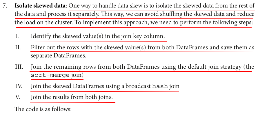
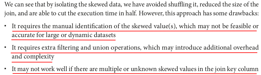
# Identify the skewed value in the invoice_id column
skewed_value = 0

# Filter out the rows with the skewed value from both DataFrames
large_skewed_df = large_df_repartitioned.filter(large_df_repartitioned.id == skewed_value)
small_skewed_df = skewed_df_repartitioned.filter(skewed_df_repartitioned.id == skewed_value)

# Filter out the rows without the skewed value from both DataFrames
large_non_skewed_df = large_df_repartitioned.filter(large_df_repartitioned.id != skewed_value)
small_non_skewed_df = skewed_df_repartitioned.filter(skewed_df_repartitioned.id != skewed_value)

# Join the non-skewed DataFrames using the default join strategy (sort-merge join)
non_skewed_join_df = large_non_skewed_df.join(small_non_skewed_df, "id")

# Join the skewed DataFrames using a broadcast hash join
skewed_join_df = large_skewed_df.join(broadcast(small_skewed_df), "id")

# Union the results from both joins
final_join_df = non_skewed_join_df.union(skewed_join_df)

measure_time(final_join_df)

 

Execution time: 6.342660903930664 seconds

 

final_join_df.explain()

 

== Physical Plan ==
Union
:- *(5) Project [id#0L, value#2, value#7]
:  +- *(5) SortMergeJoin [id#0L], [id#10L], Inner
:     :- *(2) Sort [id#0L ASC NULLS FIRST], false, 0
:     :  +- Exchange hashpartitioning(id#0L, 200), REPARTITION_BY_NUM, [plan_id=264]
:     :     +- *(1) Filter NOT (id#0L = 0)
:     :        +- *(1) Project [id#0L, rand(42) AS value#2]
:     :           +- *(1) Range (0, 10000000, step=1, splits=6)
:     +- *(4) Sort [id#10L ASC NULLS FIRST], false, 0
:        +- Exchange hashpartitioning(id#10L, 200), REPARTITION_BY_NUM, [plan_id=270]
:           +- *(3) Project [CASE WHEN ((id#5L % 4) = 0) THEN 0 ELSE id#5L END AS id#10L, value#7]
:              +- *(3) Filter NOT CASE WHEN ((id#5L % 4) = 0) THEN true ELSE (id#5L = 0) END
:                 +- *(3) Project [id#5L, rand(42) AS value#7]
:                    +- *(3) Range (0, 1000000, step=1, splits=6)
+- *(8) Project [id#31L, value#2, value#7]
   +- *(8) BroadcastHashJoin [id#31L], [id#10L], Inner, BuildRight, false
      :- Exchange hashpartitioning(id#31L, 5), REPARTITION_BY_NUM, [plan_id=279]
      :  +- *(6) Filter (id#31L = 0)
      :     +- *(6) Project [id#31L, rand(42) AS value#2]
      :        +- *(6) Range (0, 10000000, step=1, splits=6)
      +- BroadcastExchange HashedRelationBroadcastMode(List(input[0, bigint, false]),false), [plan_id=283]
         +- Exchange hashpartitioning(id#10L, 5), REPARTITION_BY_NUM, [plan_id=282]
            +- *(7) Project [CASE WHEN ((id#32L % 4) = 0) THEN 0 ELSE id#32L END AS id#10L, value#7]
               +- *(7) Filter CASE WHEN ((id#32L % 4) = 0) THEN true ELSE (id#32L = 0) END
                  +- *(7) Project [id#32L, rand(42) AS value#7]
                     +- *(7) Range (0, 1000000, step=1, splits=6)

 

 

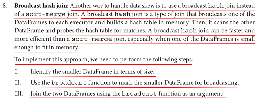
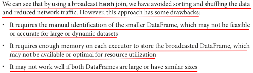
smaller_df = skewed_df_repartitioned

# Use the broadcast function to mark the smaller DataFrame for broadcasting
from pyspark.sql.functions import broadcast
broadcast_df = broadcast(smaller_df)

# Join the two DataFrames using the broadcast function as an argument

broadcast_join_df = large_df_repartitioned.join(broadcast_df, "id")

measure_time(broadcast_join_df)

 

Execution time: 3.8413877487182617 seconds

 

broadcast_join_df.explain()

 

== Physical Plan ==
*(3) Project [id#0L, value#2, value#7]
+- *(3) BroadcastHashJoin [id#0L], [id#10L], Inner, BuildRight, false
   :- Exchange hashpartitioning(id#0L, 5), REPARTITION_BY_NUM, [plan_id=365]
   :  +- *(1) Project [id#0L, rand(42) AS value#2]
   :     +- *(1) Range (0, 10000000, step=1, splits=6)
   +- BroadcastExchange HashedRelationBroadcastMode(List(input[0, bigint, false]),false), [plan_id=369]
      +- Exchange hashpartitioning(id#10L, 5), REPARTITION_BY_NUM, [plan_id=368]
         +- *(2) Project [CASE WHEN ((id#5L % 4) = 0) THEN 0 ELSE id#5L END AS id#10L, value#7]
            +- *(2) Project [id#5L, rand(42) AS value#7]
               +- *(2) Range (0, 1000000, step=1, splits=6)

 

 

spark.stop()

 

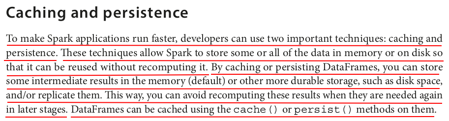
I think PySpark data frames are always in memory, so what's the need to cache or persist them?

That's a great question! It might seem like data frames in PySpark are always in memory because of Spark’s in-memory computing capabilities, but that’s not exactly the case. PySpark data frames are lazy by default, meaning that Spark doesn’t actually execute the operations until an action (like show(), collect(), or save()) is called. Instead, Spark builds up a plan of operations to be executed when an action triggers them.

Now, the need to cache or persist a data frame arises when:

1. Repeated access: If you are going to perform the same computation on a data frame multiple times (for example, performing joins, filters, or aggregations), Spark will re-compute the result each time unless you cache or persist it. Caching stores the data in memory, so Spark doesn't have to recompute the operations every time you need it.

2. Memory efficiency: If your data frame is too large to fit entirely in memory, you can persist it to disk (or a mix of memory and disk) using persist(StorageLevel) with different storage levels (like MEMORY_AND_DISK), which ensures the data is available without requiring Spark to re-read it from the original data source.

3. Avoiding recalculations: Even though operations are lazy, Spark may need to recompute intermediate results every time an action is called unless intermediate results are cached or persisted. This could cause performance issues, especially with large datasets.

In short, caching/persisting is useful when you know that a dataset will be reused and want to improve performance by keeping it available, either fully or partially, in memory (or on disk if needed).

 

from pyspark.sql import SparkSession 
from pyspark import StorageLevel 
from pyspark.sql.functions import rand, current_date, date_sub

spark = (SparkSession.builder
         .appName("cache-and-persist")
         .master("spark://ZZHPC:7077")
         .getOrCreate())

spark.sparkContext.setLogLevel("ERROR")

 

import time

def measure_time(query):
    start = time.time()
    query.collect() # Force the query execution by calling an action
    end = time.time()
    print(f"Execution time: {end - start} seconds")

 

large_df = (spark.range(0, 10000000)
            .withColumn("date", date_sub(current_date(), (rand() * 365).cast("int")))
            .withColumn("ProductId", (rand() * 100).cast("int")))
large_df.show(5)

 

+---+----------+---------+
| id|      date|ProductId|
+---+----------+---------+
|  0|2024-05-17|       28|
|  1|2025-01-11|       59|
|  2|2024-12-15|       50|
|  3|2024-05-12|       16|
|  4|2024-11-10|       89|
+---+----------+---------+
only showing top 5 rows

 

large_df.storageLevel

 

StorageLevel(False, False, False, False, 1)

 

print(large_df.storageLevel)

 

Serialized 1x Replicated

 

large_df.explain()

 

== Physical Plan ==
*(1) Project [id#0L, date#2, cast((rand(2935273770389579843) * 100.0) as int) AS ProductId#5]
+- *(1) Project [id#0L, date_sub(2025-02-08, cast((rand(-8591050805643511575) * 365.0) as int)) AS date#2]
   +- *(1) Range (0, 10000000, step=1, splits=6)

 

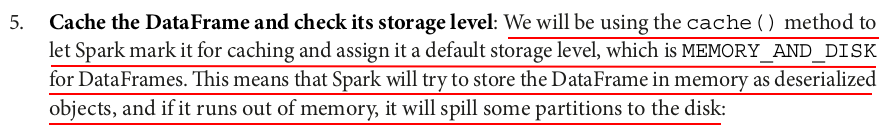
# Cache the DataFrame using cache() method
large_df.cache()

# Check the storage level of the cached DataFrame
print(large_df.storageLevel)

 

Disk Memory Deserialized 1x Replicated

 

large_df.explain()

 

== Physical Plan ==
*(1) Project [id#0L, date#2, cast((rand(2935273770389579843) * 100.0) as int) AS ProductId#5]
+- *(1) Project [id#0L, date_sub(2025-02-08, cast((rand(-8591050805643511575) * 365.0) as int)) AS date#2]
   +- *(1) Range (0, 10000000, step=1, splits=6)

Exactly the same as before.

 

# Persist the DataFrame using persist() method with a different storage level
large_df.persist(StorageLevel.MEMORY_AND_DISK_DESER)
# Check the storage level of the persisted DataFrame
print(large_df.storageLevel)

 

Disk Memory Deserialized 1x Replicated

 

large_df.explain()

 

== Physical Plan ==
*(1) Project [id#0L, date#2, cast((rand(2935273770389579843) * 100.0) as int) AS ProductId#5]
+- *(1) Project [id#0L, date_sub(2025-02-08, cast((rand(-8591050805643511575) * 365.0) as int)) AS date#2]
   +- *(1) Range (0, 10000000, step=1, splits=6)

Exactly the same as before. So StorageLevel doesn't affect execution plan.

 

help(StorageLevel)

 

Help on class StorageLevel in module pyspark.storagelevel:

class StorageLevel(builtins.object)
 |  StorageLevel(useDisk: bool, useMemory: bool, useOffHeap: bool, deserialized: bool, replication: int = 1)
 |  
 |  Flags for controlling the storage of an RDD. Each StorageLevel records whether to use memory,
 |  whether to drop the RDD to disk if it falls out of memory, whether to keep the data in memory
 |  in a JAVA-specific serialized format, and whether to replicate the RDD partitions on multiple
 |  nodes. Also contains static constants for some commonly used storage levels, MEMORY_ONLY.
 |  Since the data is always serialized on the Python side, all the constants use the serialized
 |  formats.
 |  
 |  Methods defined here:
 |  
 |  __eq__(self, other: Any) -> bool
 |      Return self==value.
 |  
 |  __init__(self, useDisk: bool, useMemory: bool, useOffHeap: bool, deserialized: bool, replication: int = 1)
 |      Initialize self.  See help(type(self)) for accurate signature.
 |  
 |  __repr__(self) -> str
 |      Return repr(self).
 |  
 |  __str__(self) -> str
 |      Return str(self).
 |  
 |  ----------------------------------------------------------------------
 |  Data descriptors defined here:
 |  
 |  __dict__
 |      dictionary for instance variables
 |  
 |  __weakref__
 |      list of weak references to the object
 |  
 |  ----------------------------------------------------------------------
 |  Data and other attributes defined here:
 |  
 |  DISK_ONLY = StorageLevel(True, False, False, False, 1)
 |  
 |  DISK_ONLY_2 = StorageLevel(True, False, False, False, 2)
 |  
 |  DISK_ONLY_3 = StorageLevel(True, False, False, False, 3)
 |  
 |  MEMORY_AND_DISK = StorageLevel(True, True, False, False, 1)
 |  
 |  MEMORY_AND_DISK_2 = StorageLevel(True, True, False, False, 2)
 |  
 |  MEMORY_AND_DISK_DESER = StorageLevel(True, True, False, True, 1)
 |  
 |  MEMORY_ONLY = StorageLevel(False, True, False, False, 1)
 |  
 |  MEMORY_ONLY_2 = StorageLevel(False, True, False, False, 2)
 |  
 |  NONE = StorageLevel(False, False, False, False, 1)
 |  
 |  OFF_HEAP = StorageLevel(True, True, True, False, 1)
 |  
 |  __annotations__ = {'DISK_ONLY': typing.ClassVar[ForwardRef('StorageLev...
 |  
 |  __hash__ = None

 

results_df = large_df.groupBy("ProductId").agg({"Id": "count"}) 
measure_time(results_df)

results_df.show(5)

 

Execution time: 2.468636989593506 seconds
+---------+---------+
|ProductId|count(Id)|
+---------+---------+
|       31|    99743|
|       85|    99814|
|       65|   100147|
|       53|    99914|
|       78|    99899|
+---------+---------+
only showing top 5 rows

 

results_df.explain()

 

== Physical Plan ==
AdaptiveSparkPlan isFinalPlan=true
+- == Final Plan ==
   *(2) HashAggregate(keys=[ProductId#5], functions=[count(1)])
   +- AQEShuffleRead coalesced
      +- ShuffleQueryStage 0
         +- Exchange hashpartitioning(ProductId#5, 200), ENSURE_REQUIREMENTS, [plan_id=69]
            +- *(1) HashAggregate(keys=[ProductId#5], functions=[partial_count(1)])
               +- InMemoryTableScan [ProductId#5]
                     +- InMemoryRelation [id#0L, date#2, ProductId#5], StorageLevel(disk, memory, deserialized, 1 replicas)
                           +- *(1) Project [id#0L, date#2, cast((rand(2935273770389579843) * 100.0) as int) AS ProductId#5]
                              +- *(1) Project [id#0L, date_sub(2025-02-08, cast((rand(-8591050805643511575) * 365.0) as int)) AS date#2]
                                 +- *(1) Range (0, 10000000, step=1, splits=6)
+- == Initial Plan ==
   HashAggregate(keys=[ProductId#5], functions=[count(1)])
   +- Exchange hashpartitioning(ProductId#5, 200), ENSURE_REQUIREMENTS, [plan_id=55]
      +- HashAggregate(keys=[ProductId#5], functions=[partial_count(1)])
         +- InMemoryTableScan [ProductId#5]
               +- InMemoryRelation [id#0L, date#2, ProductId#5], StorageLevel(disk, memory, deserialized, 1 replicas)
                     +- *(1) Project [id#0L, date#2, cast((rand(2935273770389579843) * 100.0) as int) AS ProductId#5]
                        +- *(1) Project [id#0L, date_sub(2025-02-08, cast((rand(-8591050805643511575) * 365.0) as int)) AS date#2]
                           +- *(1) Range (0, 10000000, step=1, splits=6)

 

results_df = large_df.groupBy("ProductId").agg({"Id": "count"}) 
measure_time(results_df)

results_df.show(5)

 

Execution time: 0.32273125648498535 seconds
+---------+---------+
|ProductId|count(Id)|
+---------+---------+
|       31|    99743|
|       85|    99814|
|       65|   100147|
|       53|    99914|
|       78|    99899|
+---------+---------+
only showing top 5 rows

 

results_df.storageLevel

 

StorageLevel(False, False, False, False, 1)

 

print(results_df.storageLevel)

# Serialized 1x Replicated

 

results_df.explain()

 

== Physical Plan ==
AdaptiveSparkPlan isFinalPlan=true
+- == Final Plan ==
   *(2) HashAggregate(keys=[ProductId#5], functions=[count(1)])
   +- AQEShuffleRead coalesced
      +- ShuffleQueryStage 0
         +- Exchange hashpartitioning(ProductId#5, 200), ENSURE_REQUIREMENTS, [plan_id=158]
            +- *(1) HashAggregate(keys=[ProductId#5], functions=[partial_count(1)])
               +- InMemoryTableScan [ProductId#5]
                     +- InMemoryRelation [id#0L, date#2, ProductId#5], StorageLevel(disk, memory, deserialized, 1 replicas)
                           +- *(1) Project [id#0L, date#2, cast((rand(2935273770389579843) * 100.0) as int) AS ProductId#5]
                              +- *(1) Project [id#0L, date_sub(2025-02-08, cast((rand(-8591050805643511575) * 365.0) as int)) AS date#2]
                                 +- *(1) Range (0, 10000000, step=1, splits=6)
+- == Initial Plan ==
   HashAggregate(keys=[ProductId#5], functions=[count(1)])
   +- Exchange hashpartitioning(ProductId#5, 200), ENSURE_REQUIREMENTS, [plan_id=144]
      +- HashAggregate(keys=[ProductId#5], functions=[partial_count(1)])
         +- InMemoryTableScan [ProductId#5]
               +- InMemoryRelation [id#0L, date#2, ProductId#5], StorageLevel(disk, memory, deserialized, 1 replicas)
                     +- *(1) Project [id#0L, date#2, cast((rand(2935273770389579843) * 100.0) as int) AS ProductId#5]
                        +- *(1) Project [id#0L, date_sub(2025-02-08, cast((rand(-8591050805643511575) * 365.0) as int)) AS date#2]
                           +- *(1) Range (0, 10000000, step=1, splits=6)

Exactly the same as before except the plan_id.

 

# Unpersist the DataFrame using unpersist() method
large_df.unpersist()

# Check the storage level of the unpersisted DataFrame
print(large_df.storageLevel)

 

Serialized 1x Replicated

 

spark.stop()

 

 

from pyspark.sql import SparkSession 
from pyspark.sql.functions import rand, when

spark = (SparkSession.builder
         .appName("partitioning-and-repartitioning")
         .master("spark://ZZHPC:7077")
         .getOrCreate())

spark.sparkContext.setLogLevel("ERROR")

 

large_df = (spark.range(0, 1000000)
            .withColumn("salary", 100*(rand() * 100).cast("int"))
            .withColumn("gender", when((rand() * 2).cast("int") == 0, "M").otherwise("F"))
            .withColumn("country_code", 
                        when((rand() * 4).cast("int") == 0, "US")
                        .when((rand() * 4).cast("int") == 1, "CN")
                        .when((rand() * 4).cast("int") == 2, "IN")
                        .when((rand() * 4).cast("int") == 3, "BR")))
large_df.show(5)

 

+---+------+------+------------+
| id|salary|gender|country_code|
+---+------+------+------------+
|  0|  5700|     M|          IN|
|  1|  9400|     M|        null|
|  2|  3600|     F|          BR|
|  3|  5900|     F|          US|
|  4|  1400|     F|        null|
+---+------+------+------------+
only showing top 5 rows

 

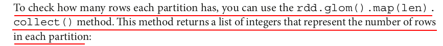
num_partitions = large_df.rdd.getNumPartitions()
print(f"Number of partitions: {num_partitions}")

partition_sizes = large_df.rdd.glom().map(len).collect()
print(f"Partition sizes: {partition_sizes}")

 

Number of partitions: 6
Partition sizes: [166666, 166667, 166667, 166666, 166667, 166667]

 

In PySpark, the rdd.glom() function is used to convert an RDD (Resilient Distributed Dataset) into a new RDD, where each element of the new RDD is an array that contains the elements of the original RDD's partitions.

To break it down:

• RDD Partitioning: Spark data is distributed across multiple partitions for parallel processing.
• Glomming: When you apply glom(), Spark collects all the elements within each partition and returns them as an array (list) in the form of a new RDD.

This function is useful when you want to view or operate on data within each partition as a whole.

For example:

rdd = sc.parallelize([1, 2, 3, 4, 5, 6], 3)  # Create an RDD with 3 partitions
glommed_rdd = rdd.glom()  # Group elements by partition
print(glommed_rdd.collect())

Output might look something like:

[[1, 2], [3, 4], [5, 6]]

Here, glom() combines the elements of each partition into a single list. This can be helpful for debugging or inspecting how the data is distributed across partitions.

Keep in mind that glom() operates on RDDs, so you would typically need to convert a DataFrame into an RDD first if you want to use glom() with DataFrames.

For DataFrame:

df.rdd.glom().collect()

This will give you the same effect but with DataFrame data.

 

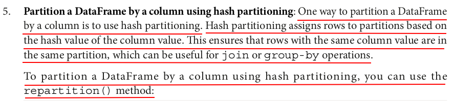
df_hash = large_df.repartition(10, "id")

 

num_partitions = df_hash.rdd.getNumPartitions()
print(f"Number of partitions: {num_partitions}")

partition_sizes = df_hash.rdd.glom().map(len).collect()
print(f"Partition sizes: {partition_sizes}")

 

Number of partitions: 10
Partition sizes: [99990, 99781, 99533, 99938, 100111, 100200, 100448, 100094, 100048, 99857]

 

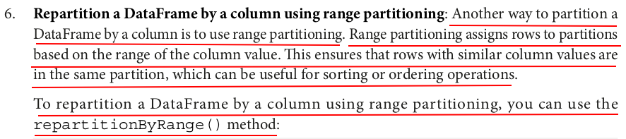
df_range = large_df.repartitionByRange(10, "id")

 

num_partitions = df_range.rdd.getNumPartitions()
print(f"Number of partitions: {num_partitions}")

partition_sizes = df_range.rdd.glom().map(len).collect()
print(f"Partition sizes: {partition_sizes}")

 

Number of partitions: 10
Partition sizes: [95015, 105687, 102164, 90999, 104296, 92395, 110608, 96219, 99349, 103268]

 

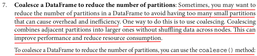
df_coalesce = df_range.coalesce(4)

 

num_partitions = df_coalesce.rdd.getNumPartitions()
print(f"Number of partitions: {num_partitions}")

partition_sizes = df_coalesce.rdd.glom().map(len).collect()
print(f"Partition sizes: {partition_sizes}")

 

Number of partitions: 4
Partition sizes: [305571, 300471, 199371, 194587]

 

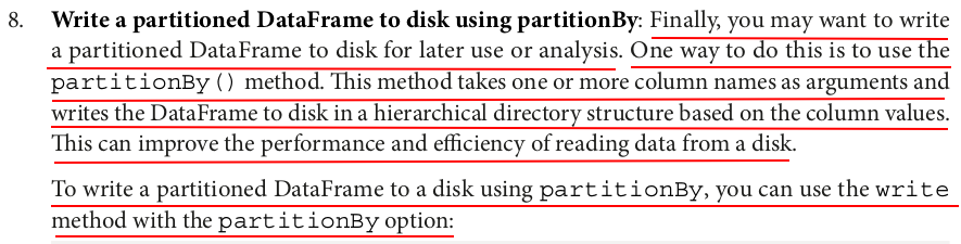
(large_df.write
    .format("parquet")
    .partitionBy("id")
    .mode("overwrite")
    .save("../data/tmp/partitioned_output"))

Files are being write to the expected location /zdata/Github/Data-Engineering-with-Databricks-Cookbook-main/data/tmp/partitioned_output. Stopped the execution because it's been running for a long time and the progress was only about 1/5.

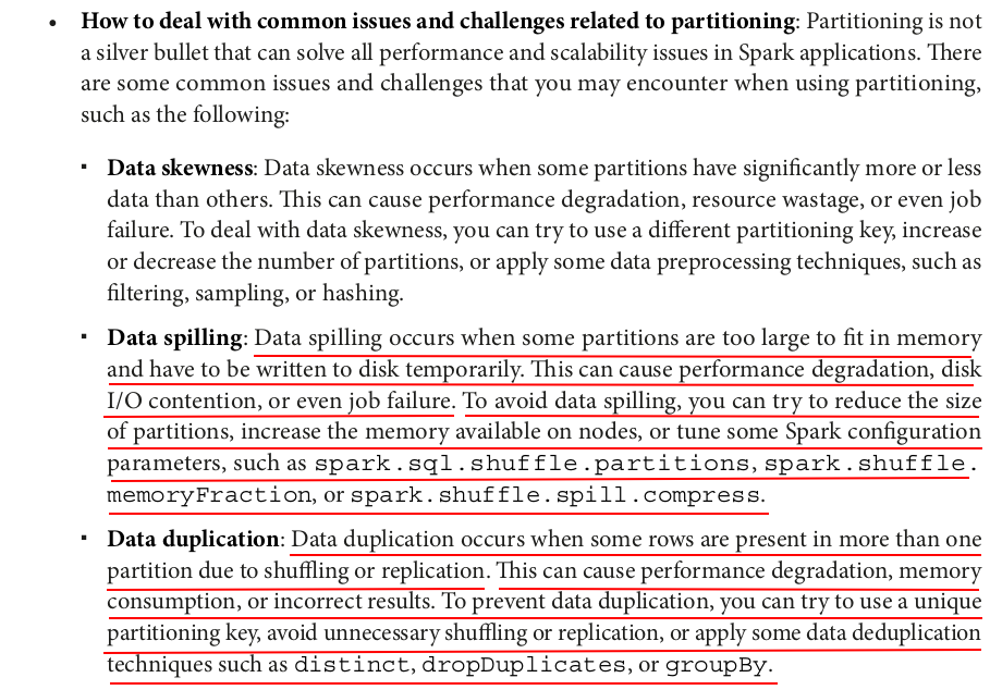
It's bad to partition by column "id" because it is unique and has a too large cardinality.

The cardinality of the partition column should not be too large or too small.

1. High Cardinality Partitioning (Many Unique Values)

• Pros:

  • Reduces data scanned for queries that filter on this column.
  • Helps in parallelizing jobs if the number of partitions is well-balanced.

• Cons:

  • Creates too many small files, leading to inefficiency in file systems like HDFS.
  • Increases metadata overhead (tracking too many partitions).
  • Might lead to small partition problem, where each task processes very little data, increasing job overhead.

Example: Partitioning by user_id in a system with millions of users is inefficient since it creates too many small partitions.

2. Low Cardinality Partitioning (Few Unique Values)

• Pros:

  • Reduces the number of partitions, making it easier to manage metadata.
  • Works well if queries often filter by this column.

• Cons:

  • Partitions may be too large, causing skewed workloads.
  • Some tasks may process too much data, leading to bottlenecks.

Example: Partitioning by country in a dataset with only a few countries might result in some partitions being too large.

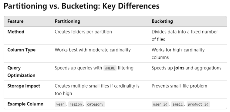
Best Practice: Choose a Column with Moderate Cardinality

• Ideal partitioning column should have a reasonable number of unique values (e.g., tens to thousands, not millions).
• Good candidates: year, month, region, department_id, etc.
• Bad candidates: transaction_id, user_id (too high), or status_flag (too low).

Alternative Approaches

• Bucketizing (bucketBy): If you need partition-like benefits but have high cardinality, consider bucketing.
• Dynamic Partitioning: If the data varies over time, dynamic partitioning can help optimize storage.

 

1. Partitioning in PySpark

Partitioning divides the data into separate directories based on a column's value, improving query efficiency for filter-based queries.

Example: Partitioning by a Column

from pyspark.sql import SparkSession

# Initialize Spark session
spark = SparkSession.builder.appName("PartitioningVsBucketing").getOrCreate()

# Sample data
data = [
    (1, "Alice", "HR", 2023),
    (2, "Bob", "Finance", 2023),
    (3, "Charlie", "HR", 2024),
    (4, "David", "Finance", 2024),
    (5, "Eve", "IT", 2023),
]

# Create DataFrame
df = spark.createDataFrame(data, ["id", "name", "department", "year"])

# Write data partitioned by 'year'
df.write.mode("overwrite").partitionBy("year").parquet("partitioned_data")

# Read partitioned data
df_partitioned = spark.read.parquet("partitioned_data")
df_partitioned.show()

What Happens?

• The data is split into directories by year (2023, 2024).
• Queries filtering by year only scan relevant partitions, reducing data scanned.

2. Bucketing in PySpark

Bucketing splits data into a fixed number of files, but unlike partitioning, it does not create directories. Instead, rows are assigned to a fixed number of buckets using a hash function.

Example: Bucketing by a Column

# Write data bucketed by 'department' into 2 buckets
df.write.mode("overwrite").bucketBy(2, "department").sortBy("id").saveAsTable("bucketed_table")

# Read bucketed table
df_bucketed = spark.sql("SELECT * FROM bucketed_table")
df_bucketed.show()

What Happens?

• Data is split into 2 buckets based on a hash of department.
• Unlike partitioning, files remain in the same directory.
• Spark does not know about buckets automatically; queries benefit when bucketed joins are used.

Steps for a Bucketed Join

1. Write Data with Bucketing – Use .bucketBy(num_buckets, "join_column") when saving tables.
2. Ensure Both Tables Have the Same Number of Buckets – Bucketing only works if both datasets use the same number of buckets.
3. Use sortBy() for Better Performance – Sorting within each bucket optimizes join performance.
4. Read the Data as a Hive Table – Bucketing benefits only apply when reading from a Hive table.

 

 

zzh@ZZHPC:/zdata/Github/Data-Engineering-with-Databricks-Cookbook-main/data/tmp/partitioned_output/_temporary/0/_temporary/attempt_202502082147112178084548336495378_0013_m_000001_38$ ls -lht | head -5
total 482M
drwxr-xr-x 2 zzh zzh 4.0K Feb  8 22:00 id=623299
drwxr-xr-x 2 zzh zzh 4.0K Feb  8 22:00 id=623294
drwxr-xr-x 2 zzh zzh 4.0K Feb  8 22:00 id=623291
drwxr-xr-x 2 zzh zzh 4.0K Feb  8 22:00 id=623288
(zpy311) zzh@ZZHPC:/zdata/Github/Data-Engineering-with-Databricks-Cookbook-main/data/tmp/partitioned_output/_temporary/0/_temporary/attempt_202502082147112178084548336495378_0013_m_000001_38$ ls -1 | wc -l
101963

zzh@ZZHPC:/zdata/Github/Data-Engineering-with-Databricks-Cookbook-main/data/tmp/partitioned_output/_temporary/0/_temporary/attempt_202502082147112178084548336495378_0013_m_000000_37$ ls -lht | head -5
total 499M
drwxr-xr-x 2 zzh zzh 4.0K Feb  8 22:01 id=127739
drwxr-xr-x 2 zzh zzh 4.0K Feb  8 22:01 id=127733
drwxr-xr-x 2 zzh zzh 4.0K Feb  8 22:01 id=127728
drwxr-xr-x 2 zzh zzh 4.0K Feb  8 22:01 id=127714
zzh@ZZHPC:/zdata/Github/Data-Engineering-with-Databricks-Cookbook-main/data/tmp/partitioned_output/_temporary/0/_temporary/attempt_202502082147112178084548336495378_0013_m_000000_37$ ls -1 | wc -l
129693

 

Reduced the records to 10000:

large_df = (spark.range(0, 10000)
            .withColumn("salary", 100*(rand() * 100).cast("int"))
            .withColumn("gender", when((rand() * 2).cast("int") == 0, "M").otherwise("F"))
            .withColumn("country_code", 
                        when((rand() * 4).cast("int") == 0, "US")
                        .when((rand() * 4).cast("int") == 1, "CN")
                        .when((rand() * 4).cast("int") == 2, "IN")
                        .when((rand() * 4).cast("int") == 3, "BR")))

Ran all the before steps.

Reran this step and it took about 25s to complete.

(zpy311) zzh@ZZHPC:~/zd/Github/Data-Engineering-with-Databricks-Cookbook-main/data/tmp/partitioned_output$ ls -lht | head -10
total 40M
-rw-r--r-- 1 zzh zzh    0 Feb  8 22:12 _SUCCESS
drwxr-xr-x 2 zzh zzh 4.0K Feb  8 22:12 id=6665
drwxr-xr-x 2 zzh zzh 4.0K Feb  8 22:12 id=6664
drwxr-xr-x 2 zzh zzh 4.0K Feb  8 22:12 id=6663
drwxr-xr-x 2 zzh zzh 4.0K Feb  8 22:12 id=6662
drwxr-xr-x 2 zzh zzh 4.0K Feb  8 22:12 id=6661
drwxr-xr-x 2 zzh zzh 4.0K Feb  8 22:12 id=6660
drwxr-xr-x 2 zzh zzh 4.0K Feb  8 22:12 id=1665
drwxr-xr-x 2 zzh zzh 4.0K Feb  8 22:12 id=6659

 

df_read = (spark.read
           .format("parquet")
           .load("../data/tmp/partitioned_output"))

df_read.show(5)

 

+------+------+------------+----+
|salary|gender|country_code|  id|
+------+------+------------+----+
|  7400|     F|          IN|1209|
|  4500|     F|          US|2609|
|  3800|     F|          US|6494|
|  4400|     F|          CN|1168|
|  5800|     F|          CN|5590|
+------+------+------------+----+
only showing top 5 rows

It took about 10s to return the result.

 

spark.stop()

 

 

from pyspark.sql import SparkSession
from pyspark.sql.functions import broadcast, col, rand, skewness,lit

spark = (SparkSession.builder
         .appName("optimize-join-strategies")
         .master("spark://ZZHPC:7077")
         .getOrCreate())

spark.sparkContext.setLogLevel("ERROR")

 

# A large data frame with 10 million rows and two columns: id and value
large_df = spark.range(0, 1000000).withColumn("value", rand(seed=42))

# A small data frame with 10000 rows and two columns: id and name
small_df = spark.range(0, 10000).withColumn("name", col("id").cast("string"))

# A skewed data frame with 10 million rows and two columns: id and value
# The id column has a Zipf distribution with a skewness of 4.7
skewed_df = spark.range(0, 1000000).withColumn("value", rand(seed=42)).withColumn("id", col("id") ** 4)

 

import time

def measure_time(query):
    start = time.time()
    query.collect() # Force the query execution by calling an action
    end = time.time()
    print(f"Execution time: {end - start} seconds")

 

In PySpark, the collect() function of a DataFrame retrieves all the rows from the distributed dataset and brings them to the driver node as a list of Row objects.

Key Points:

• It pulls all the data into memory on the driver, which can cause memory issues if the dataset is too large.
• It is useful for debugging or when you need to perform operations that require local access to all records.
• Since PySpark operates on a distributed system, collect() forces an action that triggers computation.

Alternative for Large Datasets:

• Instead of collect(), consider using take(n) or show(n, truncate=False) to avoid overloading the driver.
• Use toPandas() if you want to convert a DataFrame to a Pandas DataFrame but be cautious with large datasets.

 

 

 

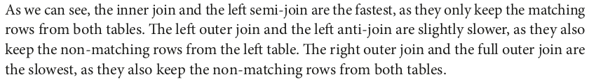
# inner join
measure_time(large_df.join(small_df, "id"))

# left outer join
measure_time(large_df.join(small_df, "id", "left"))

# right outer join
measure_time(large_df.join(small_df, "id", "right"))

# full outer join
measure_time(large_df.join(small_df, "id", "full"))

# left semi join
measure_time(large_df.join(small_df, "id", "left_semi"))

# left anti join
measure_time(large_df.join(small_df, "id", "left_anti"))

 

Execution time: 0.47536611557006836 seconds
Execution time: 2.794060707092285 seconds
Execution time: 1.6554415225982666 seconds
Execution time: 3.549330234527588 seconds
Execution time: 0.4605393409729004 seconds
Execution time: 2.3202967643737793 seconds

 

 

spark.conf.set("spark.sql.adaptive.enabled", "false")
spark.conf.set("spark.sql.autoBroadcastJoinThreshold", -1)

# Join large_df and small_df using an inner join without broadcasting
measure_time(large_df.join(small_df, "id"))

# Join large_df and small_df using an inner join with broadcasting
measure_time(large_df.join(broadcast(small_df), "id"))

 

Execution time: 2.2750749588012695 seconds
Execution time: 0.3655130863189697 seconds

 

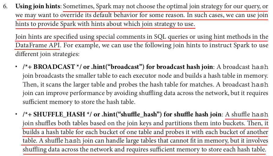
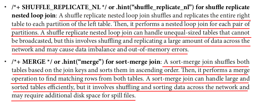
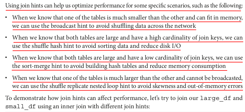
# inner join with broadcast hash join hint
inner_join_broadcast_hint = large_df.hint("broadcast").join(small_df, "id")
measure_time(inner_join_broadcast_hint)

# inner join with shuffle hash join hint
inner_join_shuffle_hash_hint = large_df.hint("shuffle_hash").join(small_df, "id")
measure_time(inner_join_shuffle_hash_hint)

# inner join with shuffle replicate nested loop join hint
inner_join_shuffle_replicate_nl_hint = large_df.hint("shuffle_replicate_nl").join(small_df, "id")
measure_time(inner_join_shuffle_replicate_nl_hint)

# inner join with sort merge join hint
inner_join_merge_hint = large_df.hint("merge").join(small_df, "id")
measure_time(inner_join_merge_hint)

 

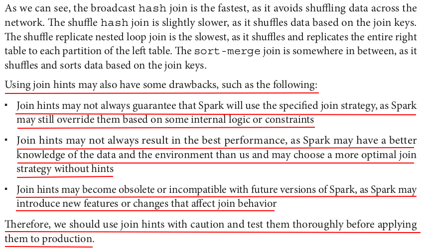
Execution time: 0.8234362602233887 seconds
Execution time: 1.34470796585083 seconds
Execution time: 83.3451840877533 seconds
Execution time: 1.246138095855713 seconds

 

 

# Join large_df and skewed_df using an inner join without AQE
spark.conf.set("spark.sql.adaptive.enabled", "false")
inner_join_no_aqe = large_df.join(skewed_df, "id")
measure_time(inner_join_no_aqe)

# Join large_df and skewed_df using an inner join with AQE
spark.conf.set("spark.sql.adaptive.enabled", "true")
inner_join_aqe = large_df.join(skewed_df, "id")
measure_time(inner_join_aqe)

 

Execution time: 1.7243151664733887 seconds
Execution time: 0.7676525115966797 seconds

 

spark.stop()