PySpark - Study Notes 2

 

 

 

 

 

For the purpose of this book, we use the Docker version of PySpark, running on a single machine. If you have a version of PySpark installed on a distributed system, we encourage using it to unleash the power of parallel computing. There is no difference in programming or commands between running your operations on a single standalone machine and doing so on a cluster. Keep in mind that you will lose out on the processing speeds if you are using a single machine.

 

 

from pyspark.sql import SparkSession
spark=SparkSession.builder.appName("Data_Wrangling").getOrCreate()

Note T he preceding step is universal for any PySpark program.

 

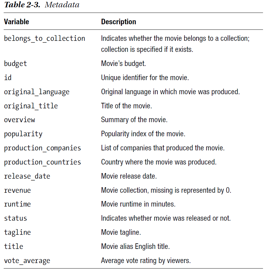
file_location = "data/C02/movie_data_part1.csv"
file_type = "csv"
infer_schema = "False"
first_row_is_header = "True"
delimiter = "|"

df = spark.read.format(file_type) \
    .option("inferSchema", infer_schema) \
    .option("header", first_row_is_header) \
    .option("sep", delimiter) \
    .load(file_location)

 

 

 

df.printSchema()

 

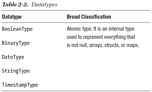
root
 |-- belongs_to_collection: string (nullable = true)
 |-- budget: string (nullable = true)
 |-- id: string (nullable = true)
 |-- original_language: string (nullable = true)
 |-- original_title: string (nullable = true)
 |-- overview: string (nullable = true)
 |-- popularity: string (nullable = true)
 |-- production_companies: string (nullable = true)
 |-- production_countries: string (nullable = true)
 |-- release_date: string (nullable = true)
 |-- revenue: string (nullable = true)
 |-- runtime: string (nullable = true)
 |-- status: string (nullable = true)
 |-- tagline: string (nullable = true)
 |-- title: string (nullable = true)
 |-- vote_average: string (nullable = true)

 

df.dtypes

 

[('belongs_to_collection', 'string'),
 ('budget', 'string'),
 ('id', 'string'),
 ('original_language', 'string'),
 ('original_title', 'string'),
 ('overview', 'string'),
 ('popularity', 'string'),
 ('production_companies', 'string'),
 ('production_countries', 'string'),
 ('release_date', 'string'),
 ('revenue', 'string'),
 ('runtime', 'string'),
 ('status', 'string'),
 ('tagline', 'string'),
 ('title', 'string'),
 ('vote_average', 'string')]

 

df.columns

 

['belongs_to_collection',
 'budget',
 'id',
 'original_language',
 'original_title',
 'overview',
 'popularity',
 'production_companies',
 'production_countries',
 'release_date',
 'revenue',
 'runtime',
 'status',
 'tagline',
 'title',
 'vote_average']

 

df.count()

# 43998

 

select_columns=['id', 'budget', 'popularity', 'release_date', 'revenue', 'title']

df = df.select(*select_columns)
df.show()

 

+-----+-------+------------------+------------+-------+--------------------+
|   id| budget|        popularity|release_date|revenue|               title|
+-----+-------+------------------+------------+-------+--------------------+
|43000|      0|             2.503|  1962-05-23|      0|The Elusive Corporal|
|43001|      0|              5.51|  1962-11-12|      0|  Sundays and Cybele|
|43002|      0|              5.62|  1962-05-24|      0|Lonely Are the Brave|
|43003|      0|             7.159|  1975-03-12|      0|          F for Fake|
|43004| 500000|             3.988|  1962-10-09|      0|Long Day's Journe...|
|43006|      0|             3.194|  1962-03-09|      0|           My Geisha|
|43007|      0|             2.689|  1962-10-31|      0|Period of Adjustment|
|43008|      0|             6.537|  1959-03-13|      0|    The Hanging Tree|
|43010|      0|             4.297|  1962-01-01|      0|Sherlock Holmes a...|
|43011|      0|             4.417|  1962-01-01|      0|  Sodom and Gomorrah|
|43012|7000000|4.7219999999999995|  1962-11-21|4000000|         Taras Bulba|
|43013|      0|             2.543|  1962-04-17|      0|The Counterfeit T...|
|43014|      0|             4.303|  1962-10-24|      0|     Tower of London|
|43015|      0|             3.493|  1962-12-07|      0|Varan the Unbelie...|
|43016|      0|             2.851|  1962-01-01|      0|Waltz of the Tore...|
|43017|      0|             4.047|  1961-10-11|      0|         Back Street|
|43018|      0|             2.661|  1961-06-02|      0|Gidget Goes Hawaiian|
|43019|      0|             3.225|  2010-05-28|      0|Schuks Tshabalala...|
|43020|      0|              5.72|  1961-06-15|      0|The Colossus of R...|
|43021|      0|             3.292|  2008-08-22|      0|          Sex Galaxy|
+-----+-------+------------------+------------+-------+--------------------+
only showing top 20 rows

 

df.select('id', 'budget', 'popularity', 'release_date', 'revenue', 'title').show()

Same result as above.

 

You also have the option of selecting the columns by index instead of selecting the names from the original DataFrame:

df.select(df[2],df[1],df[6],df[9],df[10],df[14]).show()

 

 

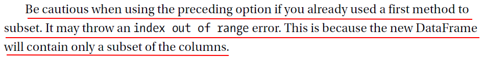
df.select(df[2],df[1],df[6],df[9],df[10],df[14]).show()

---------------------------------------------------------------------------
IndexError                                Traceback (most recent call last)
Cell In[12], line 1
----> 1 df.select(df[2],df[1],df[6],df[9],df[10],df[14]).show()

File /usr/local/spark/python/pyspark/sql/dataframe.py:3081, in DataFrame.__getitem__(self, item)
   3079     return self.select(*item)
   3080 elif isinstance(item, int):
-> 3081     jc = self._jdf.apply(self.columns[item])
   3082     return Column(jc)
   3083 else:

IndexError: list index out of range

 

df.show(25,False)


+-----+-------+------------------+------------+-------+--------------------------------------------------------+
|id   |budget |popularity        |release_date|revenue|title                                                   |
+-----+-------+------------------+------------+-------+--------------------------------------------------------+
|43000|0      |2.503             |1962-05-23  |0      |The Elusive Corporal                                    |
|43001|0      |5.51              |1962-11-12  |0      |Sundays and Cybele                                      |
|43002|0      |5.62              |1962-05-24  |0      |Lonely Are the Brave                                    |
|43003|0      |7.159             |1975-03-12  |0      |F for Fake                                              |
|43004|500000 |3.988             |1962-10-09  |0      |Long Day's Journey Into Night                           |
|43006|0      |3.194             |1962-03-09  |0      |My Geisha                                               |
|43007|0      |2.689             |1962-10-31  |0      |Period of Adjustment                                    |
|43008|0      |6.537             |1959-03-13  |0      |The Hanging Tree                                        |
|43010|0      |4.297             |1962-01-01  |0      |Sherlock Holmes and the Deadly Necklace                 |
|43011|0      |4.417             |1962-01-01  |0      |Sodom and Gomorrah                                      |
|43012|7000000|4.7219999999999995|1962-11-21  |4000000|Taras Bulba                                             |
|43013|0      |2.543             |1962-04-17  |0      |The Counterfeit Traitor                                 |
|43014|0      |4.303             |1962-10-24  |0      |Tower of London                                         |
|43015|0      |3.493             |1962-12-07  |0      |Varan the Unbelievable                                  |
|43016|0      |2.851             |1962-01-01  |0      |Waltz of the Toreadors                                  |
|43017|0      |4.047             |1961-10-11  |0      |Back Street                                             |
|43018|0      |2.661             |1961-06-02  |0      |Gidget Goes Hawaiian                                    |
|43019|0      |3.225             |2010-05-28  |0      |Schuks Tshabalala's Survival Guide to South Africa      |
|43020|0      |5.72              |1961-06-15  |0      |The Colossus of Rhodes                                  |
|43021|0      |3.292             |2008-08-22  |0      |Sex Galaxy                                              |
|43022|0      |1.548             |1961-06-11  |0      |King of the Roaring 20's – The Story of Arnold Rothstein|
|43023|0      |3.559             |1961-01-01  |0      |Konga                                                   |
|43026|0      |3.444             |1961-12-13  |0      |Paris Belongs to Us                                     |
|43027|0      |2.512             |1961-05-05  |0      |Teen Kanya                                              |
|43028|0      |6.234             |1961-08-01  |0      |Victim                                                  |
+-----+-------+------------------+------------+-------+--------------------------------------------------------+
only showing top 25 rows

 

df.show(25,True)


+-----+-------+------------------+------------+-------+--------------------+
|   id| budget|        popularity|release_date|revenue|               title|
+-----+-------+------------------+------------+-------+--------------------+
|43000|      0|             2.503|  1962-05-23|      0|The Elusive Corporal|
|43001|      0|              5.51|  1962-11-12|      0|  Sundays and Cybele|
|43002|      0|              5.62|  1962-05-24|      0|Lonely Are the Brave|
|43003|      0|             7.159|  1975-03-12|      0|          F for Fake|
|43004| 500000|             3.988|  1962-10-09|      0|Long Day's Journe...|
|43006|      0|             3.194|  1962-03-09|      0|           My Geisha|
|43007|      0|             2.689|  1962-10-31|      0|Period of Adjustment|
|43008|      0|             6.537|  1959-03-13|      0|    The Hanging Tree|
|43010|      0|             4.297|  1962-01-01|      0|Sherlock Holmes a...|
|43011|      0|             4.417|  1962-01-01|      0|  Sodom and Gomorrah|
|43012|7000000|4.7219999999999995|  1962-11-21|4000000|         Taras Bulba|
|43013|      0|             2.543|  1962-04-17|      0|The Counterfeit T...|
|43014|      0|             4.303|  1962-10-24|      0|     Tower of London|
|43015|      0|             3.493|  1962-12-07|      0|Varan the Unbelie...|
|43016|      0|             2.851|  1962-01-01|      0|Waltz of the Tore...|
|43017|      0|             4.047|  1961-10-11|      0|         Back Street|
|43018|      0|             2.661|  1961-06-02|      0|Gidget Goes Hawaiian|
|43019|      0|             3.225|  2010-05-28|      0|Schuks Tshabalala...|
|43020|      0|              5.72|  1961-06-15|      0|The Colossus of R...|
|43021|      0|             3.292|  2008-08-22|      0|          Sex Galaxy|
|43022|      0|             1.548|  1961-06-11|      0|King of the Roari...|
|43023|      0|             3.559|  1961-01-01|      0|               Konga|
|43026|      0|             3.444|  1961-12-13|      0| Paris Belongs to Us|
|43027|      0|             2.512|  1961-05-05|      0|          Teen Kanya|
|43028|      0|             6.234|  1961-08-01|      0|              Victim|
+-----+-------+------------------+------------+-------+--------------------+
only showing top 25 rows

 

from pyspark.sql.functions import *

df.filter((df['popularity'] == '') | df['popularity'].isNull() | isnan(df['popularity'])).count()

# 215

 

df.select([count(when((col(c) == '') | col(c).isNull() | isnan(c), c)).alias(c) for c in df.columns]).show()

This command selects all the columns and runs the preceding missing checks in a loop. Then when condition is used here to subset the rows that meet the missing value criteria:

+---+------+----------+------------+-------+-----+
| id|budget|popularity|release_date|revenue|title|
+---+------+----------+------------+-------+-----+
|125|   125|       215|         221|    215|  304|
+---+------+----------+------------+-------+-----+

 

df.groupBy(df['title']).count().show()

 

+--------------------+-----+
|               title|count|
+--------------------+-----+
|   The Corn Is Green|    1|
|Meet The Browns -...|    1|
|Morenita, El Esca...|    1|
| Father Takes a Wife|    1|
|The Werewolf of W...|    1|
|My Wife Is a Gang...|    1|
|Depeche Mode: Tou...|    1|
|  A Woman Is a Woman|    1|
|History Is Made a...|    1|
|      Colombian Love|    1|
|        Ace Attorney|    1|
|     Not Like Others|    1|
|40 Guns to Apache...|    1|
|          Middle Men|    1|
|         It's a Gift|    1|
|    La Vie de Bohème|    1|
|Rasputin: The Mad...|    1|
|The Ballad of Jac...|    1|
|         How to Deal|    1|
|             Freaked|    1|
+--------------------+-----+
only showing top 20 rows

 

df.groupby(df['title']).count().sort(desc("count")).show(10, False)

 

+--------------------+-----+
|title               |count|
+--------------------+-----+
|NULL                |304  |
|Les Misérables      |8    |
|The Three Musketeers|8    |
|Cinderella          |8    |
|The Island          |7    |
|A Christmas Carol   |7    |
|Hamlet              |7    |
|Dracula             |7    |
|Frankenstein        |7    |
|Framed              |6    |
+--------------------+-----+
only showing top 10 rows

 

df_temp = df.filter((df['title'] != '') & (df['title'].isNotNull()) & (~isnan(df['title'])))
df_temp.groupby(df_temp['title']).count().filter("`count` > 4").sort(col("count").desc()).show(10, False)

 

+--------------------+-----+
|title               |count|
+--------------------+-----+
|Les Misérables      |8    |
|The Three Musketeers|8    |
|Cinderella          |8    |
|A Christmas Carol   |7    |
|The Island          |7    |
|Dracula             |7    |
|Hamlet              |7    |
|Frankenstein        |7    |
|Cleopatra           |6    |
|Beauty and the Beast|6    |
+--------------------+-----+
only showing top 10 rows

 

# The following command is to find the number of titles that are repeated four times or more
df_temp.groupby(df_temp['title']).count().filter("`count` >= 4").sort(col("count").desc()).count()

# 111

 

# The following command is to delete any temporary DataFrames that we created in the process
del df_temp

 

#Before Casting
df.dtypes

 

[('id', 'string'),
 ('budget', 'string'),
 ('popularity', 'string'),
 ('release_date', 'string'),
 ('revenue', 'string'),
 ('title', 'string')]

 

#Casting
df = df.withColumn('budget',df['budget'].cast("float"))

#After Casting
df.dtypes

 

[('id', 'string'),
 ('budget', 'float'),
 ('popularity', 'string'),
 ('release_date', 'string'),
 ('revenue', 'string'),
 ('title', 'string')]

 

from pyspark.sql.types import *

int_vars = ['id']
float_vars = ['budget', 'popularity', 'revenue']
date_vars = ['release_date']

for column in int_vars:
    df = df.withColumn(column, df[column].cast(IntegerType()))

for column in float_vars:
    df = df.withColumn(column, df[column].cast(FloatType()))

for column in date_vars:
    df = df.withColumn(column, df[column].cast(DateType()))

df.dtypes

 

[('id', 'int'),
 ('budget', 'float'),
 ('popularity', 'float'),
 ('release_date', 'date'),
 ('revenue', 'float'),
 ('title', 'string')]

 

df.show(10, False)

 

+-----+--------+----------+------------+-------+---------------------------------------+
|id   |budget  |popularity|release_date|revenue|title                                  |
+-----+--------+----------+------------+-------+---------------------------------------+
|43000|0.0     |2.503     |1962-05-23  |0.0    |The Elusive Corporal                   |
|43001|0.0     |5.51      |1962-11-12  |0.0    |Sundays and Cybele                     |
|43002|0.0     |5.62      |1962-05-24  |0.0    |Lonely Are the Brave                   |
|43003|0.0     |7.159     |1975-03-12  |0.0    |F for Fake                             |
|43004|500000.0|3.988     |1962-10-09  |0.0    |Long Day's Journey Into Night          |
|43006|0.0     |3.194     |1962-03-09  |0.0    |My Geisha                              |
|43007|0.0     |2.689     |1962-10-31  |0.0    |Period of Adjustment                   |
|43008|0.0     |6.537     |1959-03-13  |0.0    |The Hanging Tree                       |
|43010|0.0     |4.297     |1962-01-01  |0.0    |Sherlock Holmes and the Deadly Necklace|
|43011|0.0     |4.417     |1962-01-01  |0.0    |Sodom and Gomorrah                     |
+-----+--------+----------+------------+-------+---------------------------------------+
only showing top 10 rows

 

df.describe()

# DataFrame[summary: string, id: string, budget: string, popularity: string, revenue: string, title: string]

 

df.describe().show()

 

+-------+------------------+--------------------+-----------------+--------------------+--------------------+
|summary|                id|              budget|       popularity|             revenue|               title|
+-------+------------------+--------------------+-----------------+--------------------+--------------------+
|  count|             43784|               43873|            43783|               43783|               43694|
|   mean|44502.304312077475|   3736901.834963166|5.295444259579189|   9697079.597382545|            Infinity|
| stddev|27189.646588626343|1.5871814952777334E7|6.168030519208248|5.6879384496288106E7|                 NaN|
|    min|                 2|                 0.0|              0.6|                 0.0|!Women Art Revolu...|
|    max|            100988|               3.8E8|            180.0|        2.78796518E9|       시크릿 Secret|
+-------+------------------+--------------------+-----------------+--------------------+--------------------+

 

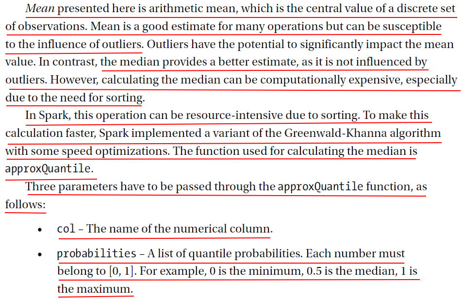
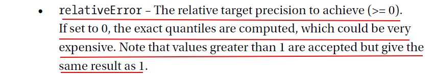
#Since unknown values in budget are marked to be 0, let's filter out those values before calculating the median
df_temp = df.filter((df['budget'] != 0) & (df['budget'].isNotNull()) & (~isnan(df['budget'])))

median = df_temp.approxQuantile('budget', [0.5], 0.1)
print('The median of budget is', median)

# The median of budget is [6000000.0]

 

# Counts the distinct occurances of titles
df.agg(countDistinct(col("title")).alias("count")).show()

Not including NULL:

+-----+
|count|
+-----+
|41138|
+-----+

 

# Counts the distinct occurrences of titles
df.select('title').distinct().count()

# 41139

Including NULL.

 

# Extracting year from the release date
df_temp  = df.withColumn('release_year', year('release_date'))
# Extracting month
df_temp = df_temp.withColumn('release_month', month('release_date'))
# Extracting day of month
df_temp = df_temp.withColumn('release_day', dayofmonth('release_date'))
# Calculating the distinct counts by the year
df_temp.groupBy("release_year").agg(countDistinct("title")).show(10, False)

 

+------------+---------------------+
|release_year|count(DISTINCT title)|
+------------+---------------------+
|1959        |271                  |
|1990        |496                  |
|1975        |365                  |
|1977        |415                  |
|1924        |19                   |
|2003        |1199                 |
|2007        |1896                 |
|2018        |4                    |
|1974        |434                  |
|2015        |13                   |
+------------+---------------------+
only showing top 10 rows

 

df.filter(df['title'].like('Meet%')).show(10,False)

 

+-----+---------+----------+------------+-----------+--------------------------+
|id   |budget   |popularity|release_date|revenue    |title                     |
+-----+---------+----------+------------+-----------+--------------------------+
|43957|500000.0 |2.649     |2005-06-28  |1000000.0  |Meet The Browns - The Play|
|39997|0.0      |3.585     |1989-11-15  |0.0        |Meet the Hollowheads      |
|16710|0.0      |11.495    |2008-03-21  |4.1939392E7|Meet the Browns           |
|20430|0.0      |3.614     |2004-01-29  |0.0        |Meet Market               |
|76435|0.0      |1.775     |2011-03-31  |0.0        |Meet the In-Laws          |
|76516|5000000.0|4.05      |1990-11-08  |485772.0   |Meet the Applegates       |
|7278 |3.0E7    |11.116    |2008-01-24  |8.4646832E7|Meet the Spartans         |
|32574|0.0      |7.42      |1941-03-14  |0.0        |Meet John Doe             |
|40506|0.0      |4.814     |1997-01-31  |0.0        |Meet Wally Sparks         |
|40688|2.4E7    |6.848     |1998-03-27  |4562146.0  |Meet the Deedles          |
+-----+---------+----------+------------+-----------+--------------------------+
only showing top 10 rows

 

df.filter(~df['title'].like('%s')).show(10, False)

 

+-----+--------+----------+------------+-------+---------------------------------------+
|id   |budget  |popularity|release_date|revenue|title                                  |
+-----+--------+----------+------------+-------+---------------------------------------+
|43000|0.0     |2.503     |1962-05-23  |0.0    |The Elusive Corporal                   |
|43001|0.0     |5.51      |1962-11-12  |0.0    |Sundays and Cybele                     |
|43002|0.0     |5.62      |1962-05-24  |0.0    |Lonely Are the Brave                   |
|43003|0.0     |7.159     |1975-03-12  |0.0    |F for Fake                             |
|43004|500000.0|3.988     |1962-10-09  |0.0    |Long Day's Journey Into Night          |
|43006|0.0     |3.194     |1962-03-09  |0.0    |My Geisha                              |
|43007|0.0     |2.689     |1962-10-31  |0.0    |Period of Adjustment                   |
|43008|0.0     |6.537     |1959-03-13  |0.0    |The Hanging Tree                       |
|43010|0.0     |4.297     |1962-01-01  |0.0    |Sherlock Holmes and the Deadly Necklace|
|43011|0.0     |4.417     |1962-01-01  |0.0    |Sodom and Gomorrah                     |
+-----+--------+----------+------------+-------+---------------------------------------+
only showing top 10 rows

 

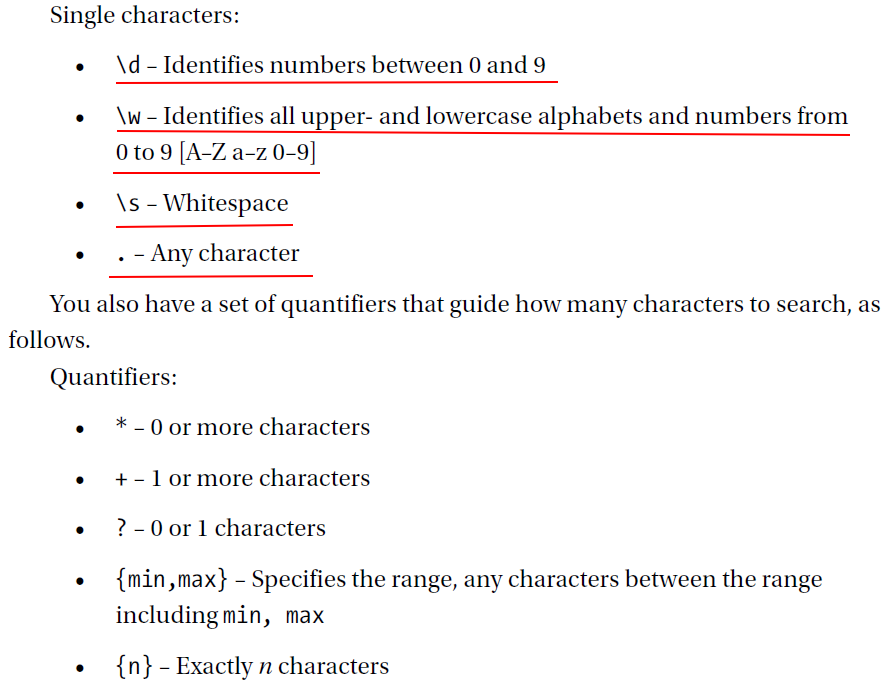
If you wanted to find any title that contains “ove,” you could use the rlike function, which is a regular expression:

df.filter(df['title'].rlike('\w*ove')).show(10, False)

 

+-----+------+----------+------------+------------+------------------------+
|id   |budget|popularity|release_date|revenue     |title                   |
+-----+------+----------+------------+------------+------------------------+
|43100|0.0   |7.252     |1959-10-07  |0.0         |General Della Rovere    |
|43152|0.0   |5.126     |2001-06-21  |0.0         |Love on a Diet          |
|43191|0.0   |4.921     |1952-08-29  |0.0         |Beware, My Lovely       |
|43281|0.0   |2.411     |1989-11-22  |0.0         |Love Without Pity       |
|43343|0.0   |3.174     |1953-12-25  |0.0         |Easy to Love            |
|43347|3.0E7 |14.863    |2010-11-22  |1.02820008E8|Love & Other Drugs      |
|43362|0.0   |1.705     |1952-02-23  |0.0         |Love Is Better Than Ever|
|43363|0.0   |2.02      |1952-05-29  |0.0         |Lovely to Look At       |
|43395|0.0   |4.758     |1950-11-10  |0.0         |Two Weeks with Love     |
|43455|0.0   |4.669     |1948-08-23  |0.0         |The Loves of Carmen     |
+-----+------+----------+------------+------------+------------------------+
only showing top 10 rows

The preceding expression can also be rewritten as follows:

df.filter(df.title.contains('ove')).show(10, False)

 

There will be situations where you’ll have thousands of columns and want to identify or subset the columns by a particular prefix or suffix. You can achieve this using the colRegex function.

df.select(df.colRegex("`re\w*`")).printSchema()

 

root
 |-- release_date: date (nullable = true)
 |-- revenue: float (nullable = true)

 

df.select(df.colRegex("`\w*e`")).printSchema()

 

root
 |-- release_date: date (nullable = true)
 |-- revenue: float (nullable = true)
 |-- title: string (nullable = true)

 

 

mean_pop = df.agg({'popularity': 'mean'}).collect()[0]['avg(popularity)']
count_obs = df.count()
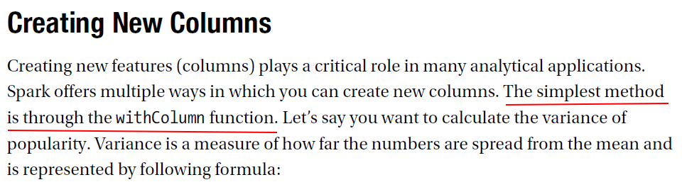
df = df.withColumn('mean_popularity', lit(mean_pop))
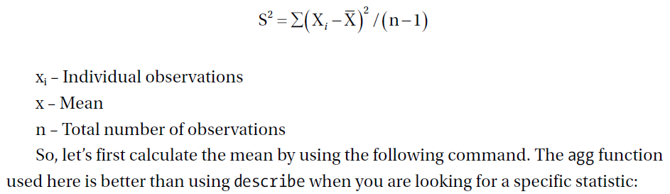
df = df.withColumn('varaiance', pow((df['popularity'] - df['mean_popularity']), 2))
variance_sum = df.agg({'varaiance': 'sum'}).collect()[0]['sum(varaiance)']
variance_population = variance_sum / (count_obs - 1)
variance_population

# 37.85868805766277

The lit() function in PySpark is used to create a column of literal values (i.e., a constant value) to be added to a DataFrame.

 

def new_cols(budget, popularity):
    if budget < 10000000:
        budget_cat = "Small"
    elif budget < 100000000:
        budget_cat = "Medium"
    else:
        budget_cat = "Big"

    if popularity < 3:
        ratings = "Low"
    elif popularity < 5:
        ratings = "Mid"
    else:
        ratings = "High"

    return budget_cat, ratings

 

# Apply the user-defined function on the DataFrame
udfB = udf(
    new_cols,
    StructType(
        [
            StructField("budget_cat", StringType(), True),
            StructField("ratings", StringType(), True),
        ]
    ),
)

 

temp_df = df.select("id", "budget", "popularity").withColumn("newcat", udfB("budget", "popularity"))

 

# Unbundle the struct type columns into individual columns and drop the struct type
df_with_newcols = temp_df.select("id", "budget", "popularity", "newcat") \
    .withColumn("budget_cat", temp_df.newcat.getItem("budget_cat")) \
    .withColumn("ratings", temp_df.newcat.getItem("ratings")) \
    .drop("newcat")

df_with_newcols.show(15, False)

 

+-----+---------+----------+----------+-------+
|id   |budget   |popularity|budget_cat|ratings|
+-----+---------+----------+----------+-------+
|43000|0.0      |2.503     |Small     |Low    |
|43001|0.0      |5.51      |Small     |High   |
|43002|0.0      |5.62      |Small     |High   |
|43003|0.0      |7.159     |Small     |High   |
|43004|500000.0 |3.988     |Small     |Mid    |
|43006|0.0      |3.194     |Small     |Mid    |
|43007|0.0      |2.689     |Small     |Low    |
|43008|0.0      |6.537     |Small     |High   |
|43010|0.0      |4.297     |Small     |Mid    |
|43011|0.0      |4.417     |Small     |Mid    |
|43012|7000000.0|4.722     |Small     |Mid    |
|43013|0.0      |2.543     |Small     |Low    |
|43014|0.0      |4.303     |Small     |Mid    |
|43015|0.0      |3.493     |Small     |Mid    |
|43016|0.0      |2.851     |Small     |Low    |
+-----+---------+----------+----------+-------+
only showing top 15 rows

Another way you can achieve the same result is using the when function.

df_with_newcols = (
    df.select("id", "budget", "popularity")
    .withColumn(
        "budget_cat",
        when(df["budget"] < 10000000, "Small")
        .when(df["budget"] < 100000000, "Medium")
        .otherwise("Big"),
    )
    .withColumn(
        "ratings",
        when(df["popularity"] < 3, "Low")
        .when(df["popularity"] < 5, "Mid")
        .otherwise("High"),
    )
)

 

columns_to_drop = ["budget_cat"]
df_with_newcols = df_with_newcols.drop(*columns_to_drop)

 

df_with_newcols = df_with_newcols.withColumnRenamed("id", "film_id").withColumnRenamed("ratings", "film_ratings")

 

new_names = [("budget", "film_budget"), ("popularity", "film_popularity")]
df_with_newcols_renamed = df_with_newcols.select(
    list(map(lambda old, new: col(old).alias(new), *zip(*new_names)))
)

 

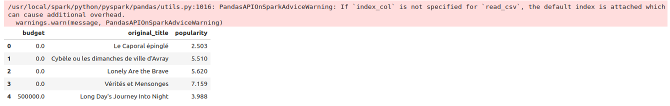
import pyspark.pandas as ps

df_pd_distributed = ps.read_csv("data/C02/movie_data_part1.csv", sep="|")
df_pd_distributed[["budget", "original_title", "popularity"]].head()

 

 

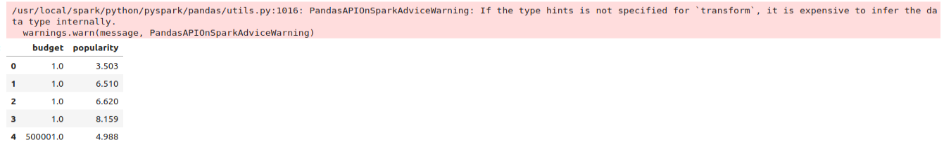
# Applying transformations on columns
import pyspark.pandas as ps


def pandas_plus(pser):
    return pser + 1  # allows an arbitrary length


df_pd_distributed_func = df_pd_distributed[["budget", "popularity"]].transform(pandas_plus)
df_pd_distributed_func.head()