


import duckdb


records = duckdb.read_csv("data/C11/Pedestrian_Counting_System_Monthly_counts_per_hour_may_2009_to_14_dec_2022.csv")
records.show(max_width=200).limit(10)

┌─────────┬───────────────────────────────┬───────┬──────────┬───────┬──────────┬───────┬───────────┬───────────────────────────────┬───────────────┐
│   ID    │           Date_Time           │ Year  │  Month   │ Mdate │   Day    │ Time  │ Sensor_ID │          Sensor_Name          │ Hourly_Counts │
│  int64  │            varchar            │ int64 │ varchar  │ int64 │ varchar  │ int64 │   int64   │            varchar            │     int64     │
├─────────┼───────────────────────────────┼───────┼──────────┼───────┼──────────┼───────┼───────────┼───────────────────────────────┼───────────────┤
│ 2887628 │ November 01, 2019 05:00:00 PM │  2019 │ November │     1 │ Friday   │    17 │        34 │ Flinders St-Spark La          │           300 │
│ 2887629 │ November 01, 2019 05:00:00 PM │  2019 │ November │     1 │ Friday   │    17 │        39 │ Alfred Place                  │           604 │
│ 2887630 │ November 01, 2019 05:00:00 PM │  2019 │ November │     1 │ Friday   │    17 │        37 │ Lygon St (East)               │           216 │
│ 2887631 │ November 01, 2019 05:00:00 PM │  2019 │ November │     1 │ Friday   │    17 │        40 │ Lonsdale St-Spring St (West)  │           627 │
│ 2887632 │ November 01, 2019 05:00:00 PM │  2019 │ November │     1 │ Friday   │    17 │        36 │ Queen St (West)               │           774 │
│ 2887633 │ November 01, 2019 05:00:00 PM │  2019 │ November │     1 │ Friday   │    17 │        29 │ St Kilda Rd-Alexandra Gardens │           644 │
│ 2887634 │ November 01, 2019 05:00:00 PM │  2019 │ November │     1 │ Friday   │    17 │        42 │ Grattan St-Swanston St (West) │           453 │
│ 2887635 │ November 01, 2019 05:00:00 PM │  2019 │ November │     1 │ Friday   │    17 │        43 │ Monash Rd-Swanston St (West)  │           387 │
│ 2887636 │ November 01, 2019 05:00:00 PM │  2019 │ November │     1 │ Friday   │    17 │        44 │ Tin Alley-Swanston St (West)  │            27 │
│ 2887637 │ November 01, 2019 05:00:00 PM │  2019 │ November │     1 │ Friday   │    17 │        35 │ Southbank                     │          2691 │
│    ·    │               ·               │    ·  │    ·     │     · │   ·      │     · │         · │     ·                         │            ·  │
│    ·    │               ·               │    ·  │    ·     │     · │   ·      │     · │         · │     ·                         │            ·  │
│    ·    │               ·               │    ·  │    ·     │     · │   ·      │     · │         · │     ·                         │            ·  │
│ 2897597 │ November 09, 2019 10:00:00 AM │  2019 │ November │     9 │ Saturday │    10 │        27 │ QV Market-Peel St             │           371 │
│ 2897598 │ November 09, 2019 10:00:00 AM │  2019 │ November │     9 │ Saturday │    10 │        28 │ The Arts Centre               │          1188 │
│ 2897599 │ November 09, 2019 10:00:00 AM │  2019 │ November │     9 │ Saturday │    10 │        31 │ Lygon St (West)               │           229 │
│ 2897600 │ November 09, 2019 10:00:00 AM │  2019 │ November │     9 │ Saturday │    10 │        30 │ Lonsdale St (South)           │           391 │
│ 2897601 │ November 09, 2019 10:00:00 AM │  2019 │ November │     9 │ Saturday │    10 │        34 │ Flinders St-Spark La          │           111 │
│ 2897602 │ November 09, 2019 10:00:00 AM │  2019 │ November │     9 │ Saturday │    10 │        37 │ Lygon St (East)               │           133 │
│ 2897603 │ November 09, 2019 10:00:00 AM │  2019 │ November │     9 │ Saturday │    10 │        40 │ Lonsdale St-Spring St (West)  │           154 │
│ 2897604 │ November 09, 2019 10:00:00 AM │  2019 │ November │     9 │ Saturday │    10 │        36 │ Queen St (West)               │           249 │
│ 2897605 │ November 09, 2019 10:00:00 AM │  2019 │ November │     9 │ Saturday │    10 │        29 │ St Kilda Rd-Alexandra Gardens │           448 │
│ 2897606 │ November 09, 2019 10:00:00 AM │  2019 │ November │     9 │ Saturday │    10 │        42 │ Grattan St-Swanston St (West) │           288 │
├─────────┴───────────────────────────────┴───────┴──────────┴───────┴──────────┴───────┴───────────┴───────────────────────────────┴───────────────┤
│ ? rows (>9999 rows, 20 shown)                                                                                                          10 columns │
└───────────────────────────────────────────────────────────────────────────────────────────────────────────────────────────────────────────────────┘
records = duckdb.read_csv(
    "data/C11/Pedestrian_Counting_System_Monthly_counts_per_hour_may_2009_to_14_dec_2022.csv",
    dtype={"Date_Time": "TIMESTAMP"},
    timestamp_format="%B %d, %Y %H:%M:%S %p",
)
records.limit(5).show(max_width=200)
┌─────────┬─────────────────────┬───────┬──────────┬───────┬─────────┬───────┬───────────┬──────────────────────────────┬───────────────┐
│   ID    │      Date_Time      │ Year  │  Month   │ Mdate │   Day   │ Time  │ Sensor_ID │         Sensor_Name          │ Hourly_Counts │
│  int64  │      timestamp      │ int64 │ varchar  │ int64 │ varchar │ int64 │   int64   │           varchar            │     int64     │
├─────────┼─────────────────────┼───────┼──────────┼───────┼─────────┼───────┼───────────┼──────────────────────────────┼───────────────┤
│ 2887628 │ 2019-11-01 17:00:00 │  2019 │ November │     1 │ Friday  │    17 │        34 │ Flinders St-Spark La         │           300 │
│ 2887629 │ 2019-11-01 17:00:00 │  2019 │ November │     1 │ Friday  │    17 │        39 │ Alfred Place                 │           604 │
│ 2887630 │ 2019-11-01 17:00:00 │  2019 │ November │     1 │ Friday  │    17 │        37 │ Lygon St (East)              │           216 │
│ 2887631 │ 2019-11-01 17:00:00 │  2019 │ November │     1 │ Friday  │    17 │        40 │ Lonsdale St-Spring St (West) │           627 │
│ 2887632 │ 2019-11-01 17:00:00 │  2019 │ November │     1 │ Friday  │    17 │        36 │ Queen St (West)              │           774 │
└─────────┴─────────────────────┴───────┴──────────┴───────┴─────────┴───────┴───────────┴──────────────────────────────┴───────────────┘
Before loading our dataset into an on-disk database for analysis, we can also consider whether there are any data transformations we may want to apply.
transformed = records.select("* EXCLUDE ID").sort("Date_Time")
transformed.limit(5).show(max_width=200)
┌─────────────────────┬───────┬─────────┬───────┬─────────┬───────┬───────────┬───────────────────────────────────┬───────────────┐
│      Date_Time      │ Year  │  Month  │ Mdate │   Day   │ Time  │ Sensor_ID │            Sensor_Name            │ Hourly_Counts │
│      timestamp      │ int64 │ varchar │ int64 │ varchar │ int64 │   int64   │              varchar              │     int64     │
├─────────────────────┼───────┼─────────┼───────┼─────────┼───────┼───────────┼───────────────────────────────────┼───────────────┤
│ 2009-05-01 00:00:00 │  2009 │ May     │     1 │ Friday  │     0 │         1 │ Bourke Street Mall (North)        │            53 │
│ 2009-05-01 00:00:00 │  2009 │ May     │     1 │ Friday  │     0 │         2 │ Bourke Street Mall (South)        │            52 │
│ 2009-05-01 00:00:00 │  2009 │ May     │     1 │ Friday  │     0 │         4 │ Town Hall (West)                  │           209 │
│ 2009-05-01 00:00:00 │  2009 │ May     │     1 │ Friday  │     0 │         5 │ Princes Bridge                    │           157 │
│ 2009-05-01 00:00:00 │  2009 │ May     │     1 │ Friday  │     0 │         6 │ Flinders Street Station Underpass │           139 │
└─────────────────────┴───────┴─────────┴───────┴─────────┴───────┴───────────┴───────────────────────────────────┴───────────────┘

with duckdb.connect("pedestrian.duckdb") as conn:
    result = (
        conn.read_csv(
            "data/C11/Pedestrian_Counting_System_Monthly_counts_per_hour_may_2009_to_14_dec_2022.csv",
            dtype={"Date_Time": "TIMESTAMP"},
            timestamp_format="%B %d, %Y %H:%M:%S %p",
        )
        .select("* EXCLUDE ID")
        .sort("Date_Time")
    )
    result.to_table("pedestrian_counts")

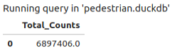
conn = duckdb.connect("pedestrian.duckdb")
conn.sql(
    """
    SELECT sum(Hourly_Counts) AS Total_Counts
    FROM pedestrian_counts
    WHERE Year = 2022 AND Sensor_Name = 'Melbourne Central'
    """
)
┌──────────────┐
│ Total_Counts │
│    int128    │
├──────────────┤
│      6897406 │
└──────────────┘
conn.close()
%load_ext sql
conn = duckdb.connect()
%sql conn --alias duckdb
conn.close()
In our context, we want to work with the database we created in the previous section; so, let’s configure JupySQL so that it uses a new connection to our on-disk pedestrian.duckdb database while also giving it an appropriate alias:
conn = duckdb.connect("pedestrian.duckdb")
%sql conn --alias pedestrian.duckdb
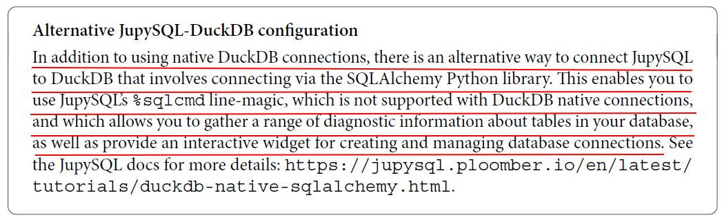
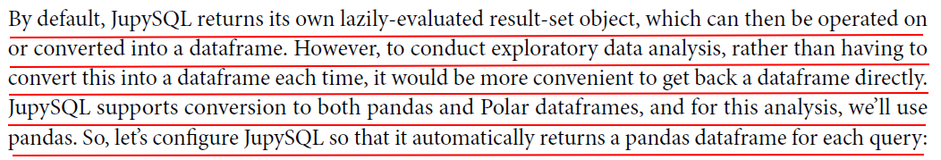
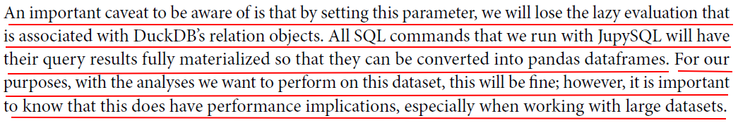
%config SqlMagic.autopandas = True
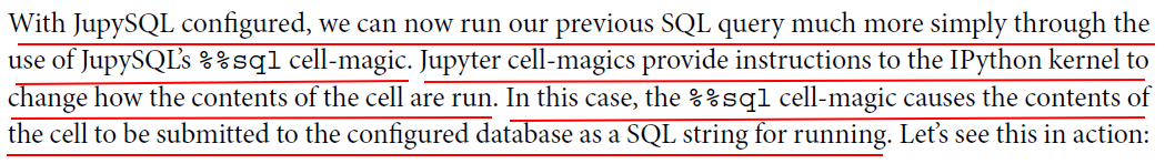
%%sql
SELECT sum(Hourly_Counts) AS Total_Counts
FROM pedestrian_counts
WHERE Year = 2022 AND Sensor_Name = 'Melbourne Central'
type(_)

# pandas.core.frame.DataFrame
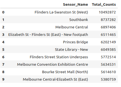
%%sql sensors_2022_df <<
SELECT Sensor_Name, sum(Hourly_Counts)::BIGINT AS Total_Counts
FROM pedestrian_counts
WHERE Year = 2022
GROUP BY Sensor_Name
ORDER BY Total_Counts DESC
sensors_2022_df.head(10)
sensors_2022_df.dtypes
Sensor_Name     object
Total_Counts     int64
dtype: object
In addition to confirming that the Total Counts column of our dataframe has an int64 data type, we can also see that the Sensor Name column contains the dtype object. While this can be a little misleading at first, this is pandas’ default way of representing string values and is therefore appropriate for this column.

import plotly.express as px
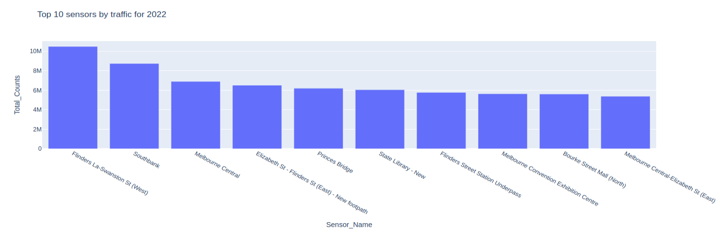
With the Plotly Express module loaded, let’s see it in action by using the px.bar() function to create a bar chart of the top 10 sensors by traffic in 2022 while using the sensors_2022_df dataframe we created in the previous section:
figure = px.bar(
    sensors_2022_df.head(10),
    x="Sensor_Name",
    y="Total_Counts",
    height=500,
    title="Top 10 sensors by traffic for 2022",
)
figure
Let’s make one more visualization with Plotly Express. This time, we’ll visualize the number of active sensors across each year using a line plot. Plotly provides this functionality through the px.line() function. First, we’ll need to query our database to get the distinct number of sensor names seen across each year, which we can do with the following DuckDB query:
%%sql sensor_years_df <<
SELECT Year, COUNT(DISTINCT Sensor_Name) AS Total_Sensors
FROM pedestrian_counts
GROUP BY Year
ORDER BY Year
sensor_years_df.head(5)
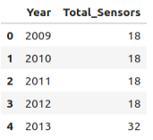
figure = px.line(
    sensor_years_df,
    x="Year",
    y="Total_Sensors",
    markers=True,
    height=500,
    title="Total number of active sensors by year"
)
figure

figure.update_layout(xaxis={"dtick": 1}, title={"x": 0.5})
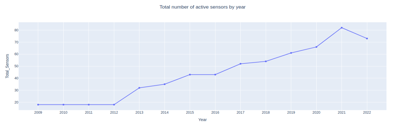
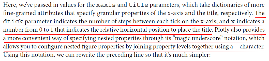
figure.update_layout(xaxis_dtick=1, title_x=0.5)
In this short introduction to making visualizations with Plotly, we’ve focused on two Plotly Express functions, as well as Plotly chart customizations via a handful of figure-layout properties; however, this is by no means a comprehensive overview of using the library. Two resources we’d recommend consulting if you want to further explore using Plotly in Python are as follows:
• The Plotly Express guide: https://plotly.com/python/plotly-express
• The Plotly Python Figure reference: https://plotly.com/python/reference/index


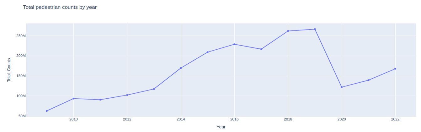
%%sql year_counts_df <<
SELECT Year, sum(Hourly_Counts)::BIGINT AS Total_Counts
FROM pedestrian_counts
GROUP BY Year
ORDER BY Year
px.line(
    year_counts_df,
    x="Year",
    y="Total_Counts",
    markers=True,
    height=500,
    title="Total pedestrian counts by year",
)
%sql SELECT count(DISTINCT Year) FROM pedestrian_counts
%%sql
CREATE OR REPLACE TABLE common_sensors AS
SELECT Sensor_Name
FROM pedestrian_counts
GROUP BY Sensor_Name
HAVING COUNT(DISTINCT Year) = 14;
Ordinarily, when issuing a CREATE TABLE statement in DuckDB, no results are returned. When using JupySQL to submit database-modifying SQL, however, it returns the number of rows that were inserted into the database. This means we’ll see the following dataframe as output:
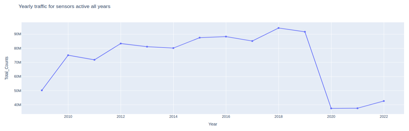
%%sql year_counts_filtered_df <<
SELECT Year, sum(Hourly_Counts)::BIGINT AS Total_Counts
FROM pedestrian_counts
WHERE Sensor_Name IN (FROM common_sensors)
GROUP BY Year
ORDER BY Year
px.line(
    year_counts_filtered_df,
    x="Year",
    y="Total_Counts",
    markers=True,
    height=500,
    title="Yearly traffic for sensors active all years",
)
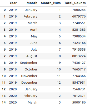
%%sql year_month_counts_df <<
SELECT Year,
    Month,
    month(Date_Time) AS Month_Num,
    sum(Hourly_Counts)::BIGINT AS Total_Counts
FROM pedestrian_counts
WHERE Year IN (2019, 2020, 2021)
  AND Sensor_Name in (FROM common_sensors)
GROUP BY Year, Month, Month_Num
ORDER BY Year, Month_Num
year_month_counts_df.head(15)
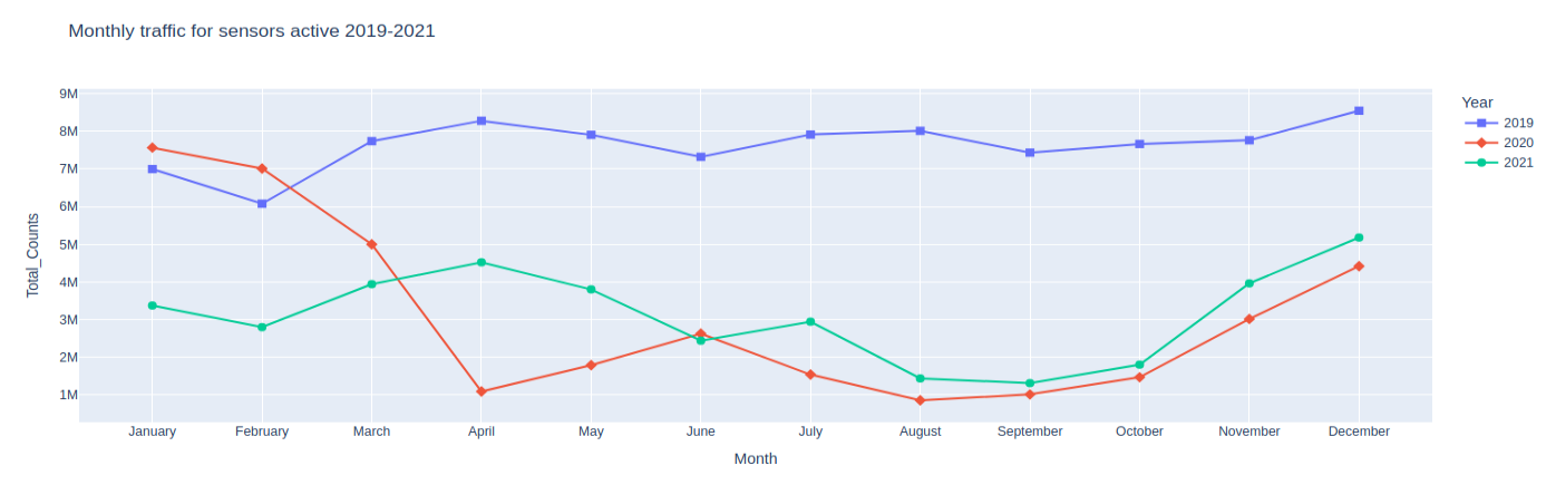
px.line(
    year_month_counts_df,
    x="Month",
    y="Total_Counts",
    color="Year",
    symbol="Year",
    symbol_sequence=["square", "diamond", "circle"],
    markers=True,
    height=500,
    title="Monthly traffic for sensors active 2019-2021",
).update_traces(marker_size=8)

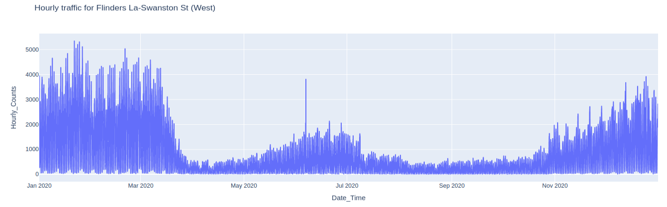
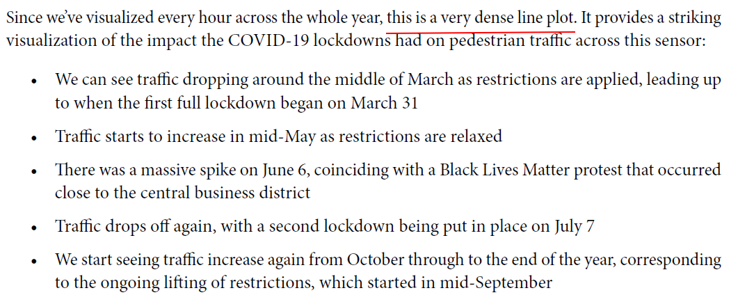
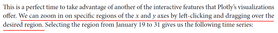
%%sql sensor_2020_df <<
SELECT Hourly_Counts, Date_Time
FROM pedestrian_counts
WHERE Sensor_Name = 'Flinders La-Swanston St (West)' AND Year = 2020
Then, we’ll use the px.line() function to create a time series plot of all readings for that year:
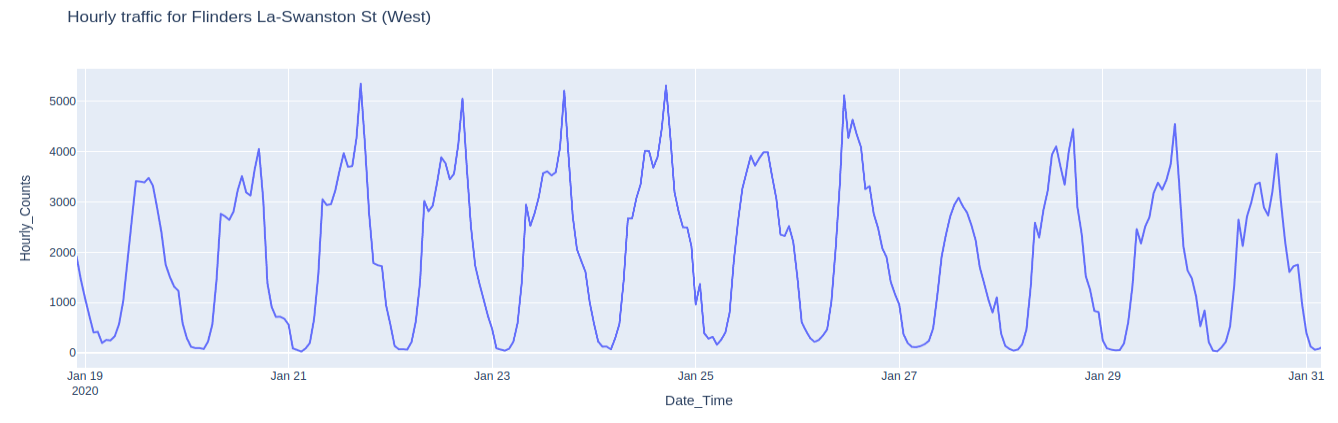
%%sql multi_sensor_df <<
SELECT Sensor_Name, Hourly_Counts, Date_Time
FROM pedestrian_counts
WHERE Sensor_Name IN (
    'Flinders St-Spark La',
    'Bourke Street Mall (North)',
    'Southern Cross Station'
) AND Year = 2019 AND Month = 'September'
px.line(
    multi_sensor_df,
    y="Hourly_Counts",
    x="Date_Time",
    facet_col="Sensor_Name",
    facet_col_wrap=1,
    title="Hourly pedestrian traffic for December 2019",
    height=800,
).update_layout(yaxis_fixedrange=True)

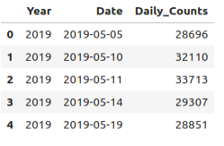
%%sql bourke_daily_df <<
SELECT Year,
    Date_Time::DATE AS Date,
    sum(Hourly_Counts)::BIGINT AS Daily_Counts,
 FROM pedestrian_counts
WHERE Sensor_Name = 'Bourke Street Mall (North)'
  AND Year IN (2019, 2020, 2021)
GROUP BY Year, Date
bourke_daily_df.head()
px.box(
    bourke_daily_df,
    x="Year",
    y="Daily_Counts",
    points="all",
    height=600,
    title="Distributions of daily traffic for a sensor",
)
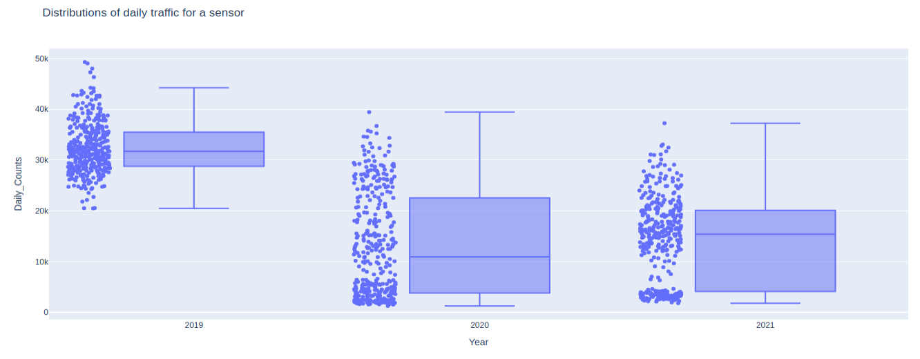


【推荐】国内首个AI IDE,深度理解中文开发场景,立即下载体验Trae
【推荐】编程新体验,更懂你的AI,立即体验豆包MarsCode编程助手
【推荐】抖音旗下AI助手豆包,你的智能百科全书,全免费不限次数
【推荐】轻量又高性能的 SSH 工具 IShell:AI 加持,快人一步
· 震惊!C++程序真的从main开始吗?99%的程序员都答错了
· 【硬核科普】Trae如何「偷看」你的代码?零基础破解AI编程运行原理
· 单元测试从入门到精通
· 上周热点回顾(3.3-3.9)
· winform 绘制太阳,地球,月球 运作规律
2024-01-16 Redis - List Use Cases
2024-01-16 Redis - HyperLogLog Use Cases
2024-01-16 Redis - SORT