Data Generation
points, directions = generate_sequences(n=128, seed=13)
And then let’s visualize the first ten squares:
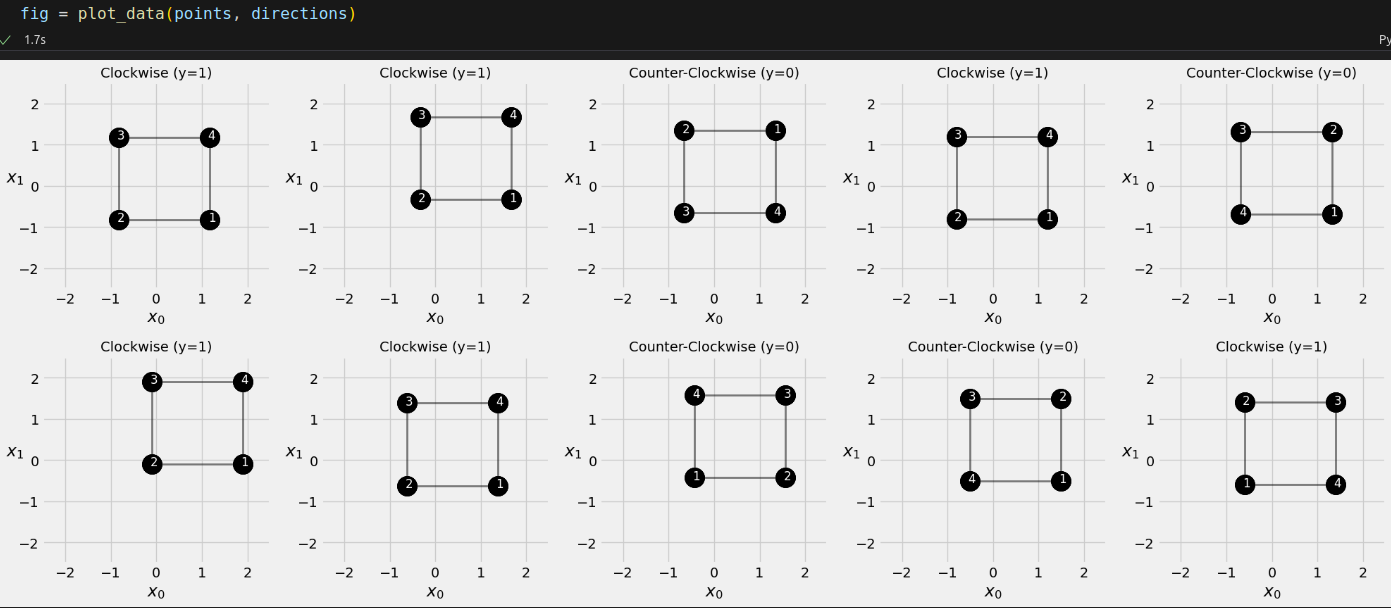
The corners show the order in which they were drawn. In the first square, the drawing started at the bottom-right corner (corresponding to the red D corner) and followed a clockwise direction (corresponding to the DABC sequence).


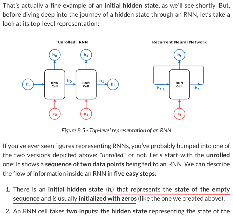
hidden_state = torch.zeros(2)
hidden_state

# tensor([0., 0.])

input_size = 2
hidden_size = 2

torch.manual_seed(19)
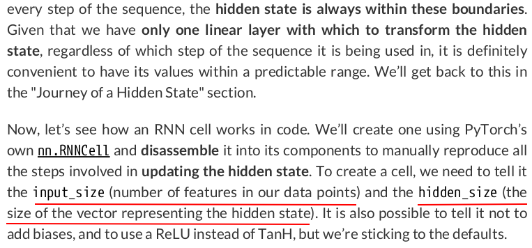
rnn_cell = nn.RNNCell(input_size=input_size, hidden_size=hidden_size)
rnn_state = rnn_cell.state_dict()
rnn_state
OrderedDict([('weight_ih',
              tensor([[ 0.6627, -0.4245],
                      [ 0.5373,  0.2294]])),
             ('weight_hh',
              tensor([[-0.4015, -0.5385],
                      [-0.1956, -0.6835]])),
             ('bias_ih', tensor([0.4954, 0.6533])),
             ('bias_hh', tensor([-0.3565, -0.2904]))])

linear_input = nn.Linear(input_size, hidden_size)
linear_hidden = nn.Linear(hidden_size, hidden_size)

with torch.no_grad():
    linear_input.weight = nn.Parameter(rnn_state['weight_ih'])
    linear_input.bias = nn.Parameter(rnn_state['bias_ih'])
    linear_hidden.weight = nn.Parameter(rnn_state['weight_hh'])
    linear_hidden.bias = nn.Parameter(rnn_state['bias_hh'])
Now, let’s work our way through the mechanics of the RNN cell! It all starts with the initial hidden state representing the empty sequence:
initial_hidden = torch.zeros(1, hidden_size)
initial_hidden

# tensor([[0., 0.]])
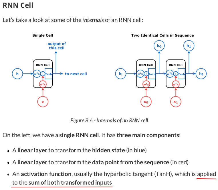
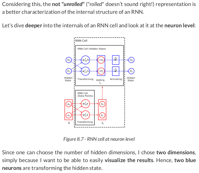
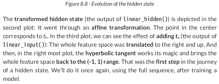
Then, we use the two blue neurons, the linear_hidden layer, to transform the hidden state:
th = linear_hidden(initial_hidden)
th

# tensor([[-0.3565, -0.2904]], grad_fn=<AddmmBackward0>)
Cool! Now, let’s take look at a sequence of data points from our dataset:
X = torch.as_tensor(points[0]).float()
X
tensor([[ 1.1767, -0.8233],
        [-0.8233, -0.8233],
        [-0.8233,  1.1767],
        [ 1.1767,  1.1767]])
As expected, four data points, two coordinates each. The first data point, [1.1767, -0.8233], corresponding to the bottom-right corner of the square, is going to be transformed by the linear_input layers (the two red neurons):
tx = linear_input(X[0:1])
tx

# tensor([[1.6247, 1.0967]], grad_fn=<AddmmBackward0>)
There we go: We got both tx and th. Let’s add them together:
adding = th + tx
adding

# tensor([[1.2681, 0.8063]], grad_fn=<AddBackward0>)
The effect of adding tx is similar to the effect of adding the bias: It is effectively translating the transformed hidden state to the right (by 1.6247) and up (by 1.0967).
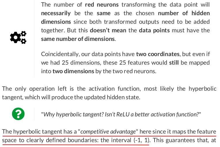
Finally, the hyperbolic tangent activation function "compresses" the feature space back into the (-1, 1) interval:
torch.tanh(adding)

# tensor([[0.8533, 0.6675]], grad_fn=<TanhBackward0>)
That’s the updated hidden state!
Now, let’s take a quick sanity check, feeding the same input to the original RNN cell:
rnn_cell(X[0:1])

# tensor([[0.8533, 0.6675]], grad_fn=<TanhBackward0>)


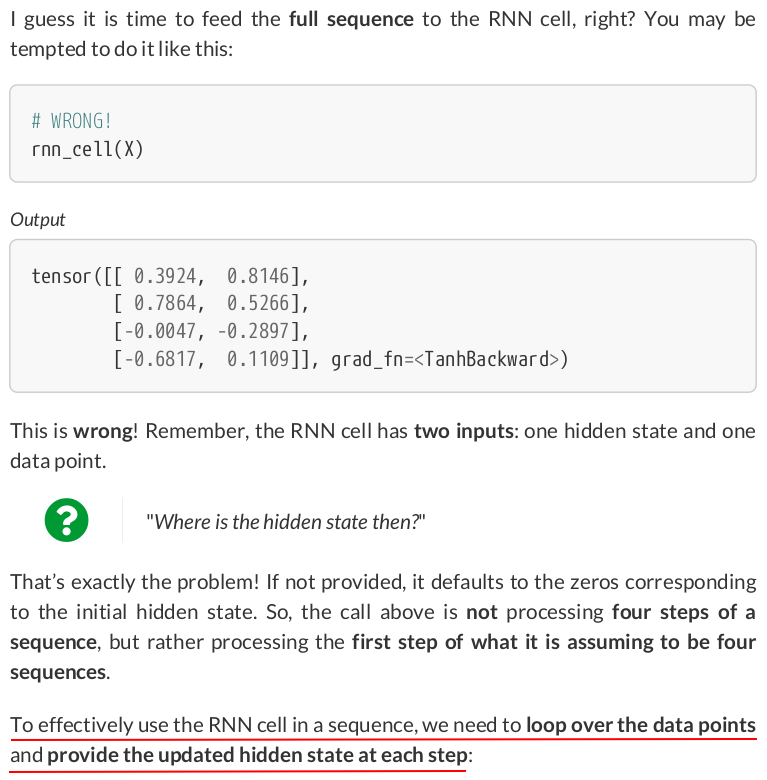
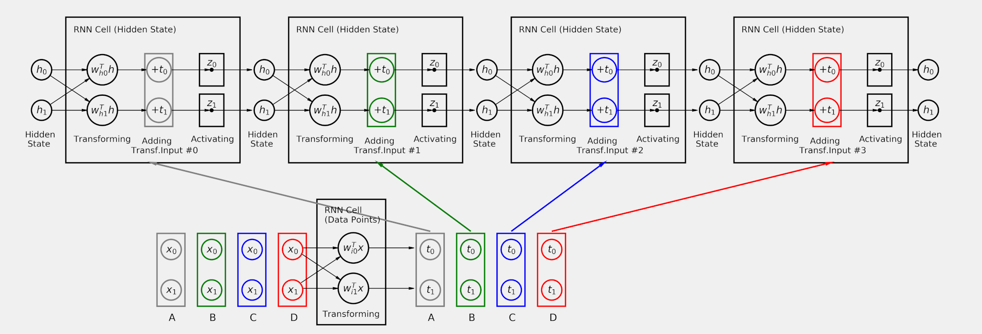
hidden = torch.zeros(1, hidden_size)
for i in range(X.shape[0]):
    out = rnn_cell(X[i:i+1], hidden)
    print(out)
    hidden = out
tensor([[0.8533, 0.6675]], grad_fn=<TanhBackward0>)
tensor([[-0.6407, -0.7121]], grad_fn=<TanhBackward0>)
tensor([[-0.2594,  0.6654]], grad_fn=<TanhBackward0>)
tensor([[0.1636, 0.6967]], grad_fn=<TanhBackward0>)
Now we’re talking! The last hidden state, (0.1636, 0.6967), is the representation of the full sequence.
input_size = 2
hidden_size = 2

torch.manual_seed(19)
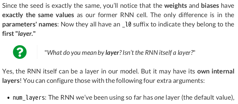
rnn = nn.RNN(input_size=input_size, hidden_size=hidden_size)
rnn.state_dict()
OrderedDict([('weight_ih_l0',
              tensor([[ 0.6627, -0.4245],
                      [ 0.5373,  0.2294]])),
             ('weight_hh_l0',
              tensor([[-0.4015, -0.5385],
                      [-0.1956, -0.6835]])),
             ('bias_ih_l0', tensor([0.4954, 0.6533])),
             ('bias_hh_l0', tensor([-0.3565, -0.2904]))])

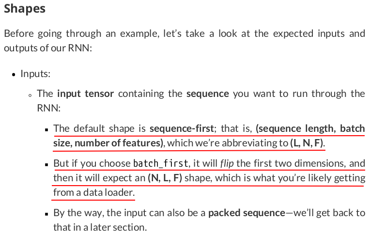
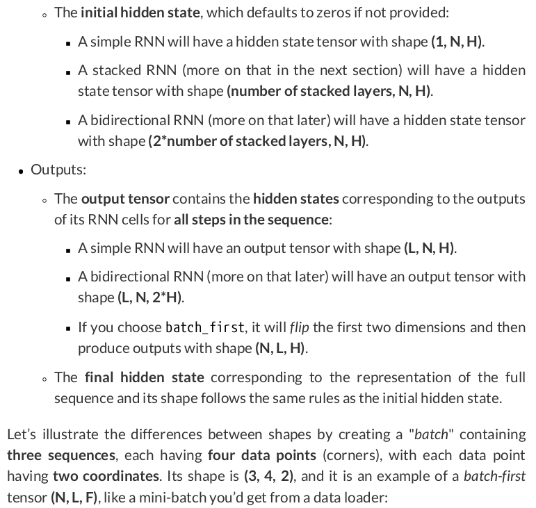
batch = torch.as_tensor(np.array(points[:3])).float()
batch.shape

# torch.Size([3, 4, 2])

permuted_batch = batch.permute(1, 0, 2)
permuted_batch.shape

# torch.Size([4, 3, 2])
Now the data is in an "RNN-friendly" shape, and we can run it through a regular RNN to get two sequence-first tensors back:
torch.manual_seed(19)
rnn = nn.RNN(input_size=input_size, hidden_size=hidden_size)
out, final_hidden = rnn(permuted_batch)
out.shape, final_hidden.shape

# (torch.Size([4, 3, 2]), torch.Size([1, 3, 2]))
For simple RNNs, the last element of the output IS the final hidden state!
(out[-1] == final_hidden).all()

# tensor(True)
Once we’re done with the RNN, we can turn the data back to our familiar batch-first shape:
batch_hidden = final_hidden.permute(1, 0, 2)
batch_hidden.shape

# torch.Size([3, 1, 2])
That seems like a lot of work, though. Alternatively, we could set the RNN’s batch_first argument to True so we can use the batch above without any modifications:
torch.manual_seed(19)
rnn_batch_first = nn.RNN(input_size=input_size, hidden_size=hidden_size, batch_first=True)
out, final_hidden = rnn_batch_first(batch)
out.shape, final_hidden.shape

# (torch.Size([3, 4, 2]), torch.Size([1, 3, 2]))
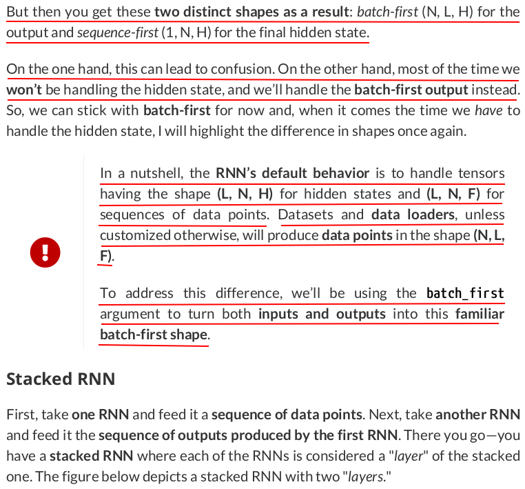
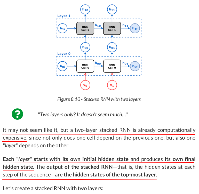
torch.manual_seed(19)
rnn_stacked = nn.RNN(input_size=2, hidden_size=2, num_layers=2, batch_first=True)
state = rnn_stacked.state_dict()
state
OrderedDict([('weight_ih_l0',
              tensor([[ 0.6627, -0.4245],
                      [ 0.5373,  0.2294]])),
             ('weight_hh_l0',
              tensor([[-0.4015, -0.5385],
                      [-0.1956, -0.6835]])),
             ('bias_ih_l0', tensor([0.4954, 0.6533])),
             ('bias_hh_l0', tensor([-0.3565, -0.2904])),
             ('weight_ih_l1',
              tensor([[-0.6701, -0.5811],
                      [-0.0170, -0.5856]])),
             ('weight_hh_l1',
              tensor([[ 0.1159, -0.6978],
                      [ 0.3241, -0.0983]])),
             ('bias_ih_l1', tensor([-0.3163, -0.2153])),
             ('bias_hh_l1', tensor([ 0.0722, -0.3242]))])

rnn_layer0 = nn.RNN(input_size=2, hidden_size=2, batch_first=True)
rnn_layer1 = nn.RNN(input_size=2, hidden_size=2, batch_first=True)

state_list = list(state.items())
rnn_layer0.load_state_dict(dict(state_list[:4]))
rnn_layer1.load_state_dict(dict([(k[:-1] + '0', v) for k, v in state_list[4:]]))

# <All keys matched successfully>
Now, let’s make a batch containing one sequence from our synthetic dataset (thus having shape (N=1, L=4, F=2)):
x = torch.as_tensor(points[0:1]).float()
The RNN representing the first layer takes the sequence of data points as usual:
out0, h0 = rnn_layer0(x)

out1, h1 = rnn_layer1(out0)

out1, torch.cat([h0, h1])
(tensor([[[-0.8348, -0.7374],
          [ 0.7686, -0.3002],
          [-0.1572, -0.5691],
          [-0.3625, -0.7376]]], grad_fn=<TransposeBackward1>),
 tensor([[[ 0.1636,  0.6967]],

         [[-0.3625, -0.7376]]], grad_fn=<CatBackward0>))
Done! We’ve replicated the inner workings of a stacked RNN using two simple RNNs. You can double-check the results by feeding the sequence of data points to the actual stacked RNN itself:
out, hidden = rnn_stacked(x)
out, hidden
(tensor([[[-0.8348, -0.7374],
          [ 0.7686, -0.3002],
          [-0.1572, -0.5691],
          [-0.3625, -0.7376]]], grad_fn=<TransposeBackward1>),
 tensor([[[ 0.1636,  0.6967]],

         [[-0.3625, -0.7376]]], grad_fn=<StackBackward0>))
And you’ll get exactly the same results.

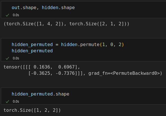
(out[:, -1] == hidden.permute(1, 0, 2)[:, -1]).all()

# tensor(True)
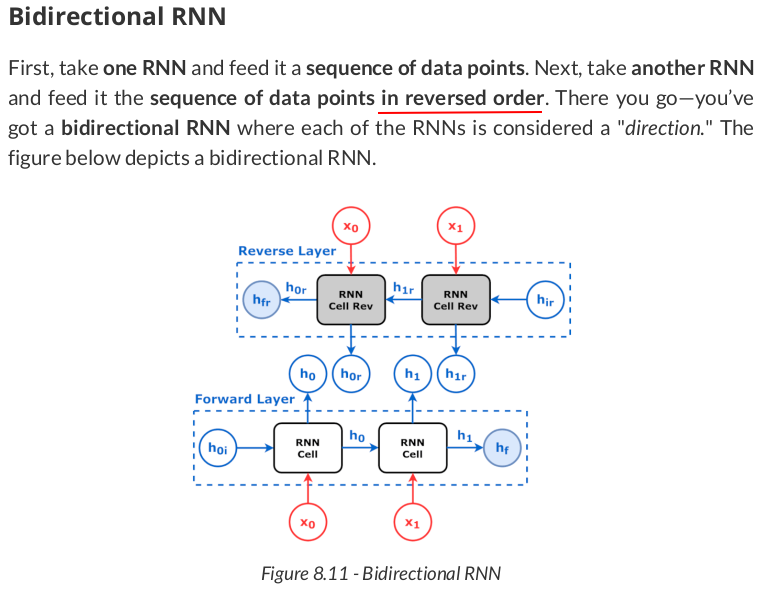
torch.manual_seed(19)
rnn_bidirect = nn.RNN(input_size=2, hidden_size=2, bidirectional=True, batch_first=True)
state = rnn_bidirect.state_dict()
state
OrderedDict([('weight_ih_l0',
              tensor([[ 0.6627, -0.4245],
                      [ 0.5373,  0.2294]])),
             ('weight_hh_l0',
              tensor([[-0.4015, -0.5385],
                      [-0.1956, -0.6835]])),
             ('bias_ih_l0', tensor([0.4954, 0.6533])),
             ('bias_hh_l0', tensor([-0.3565, -0.2904])),
             ('weight_ih_l0_reverse',
              tensor([[-0.6701, -0.5811],
                      [-0.0170, -0.5856]])),
             ('weight_hh_l0_reverse',
              tensor([[ 0.1159, -0.6978],
                      [ 0.3241, -0.0983]])),
             ('bias_ih_l0_reverse', tensor([-0.3163, -0.2153])),
             ('bias_hh_l0_reverse', tensor([ 0.0722, -0.3242]))])
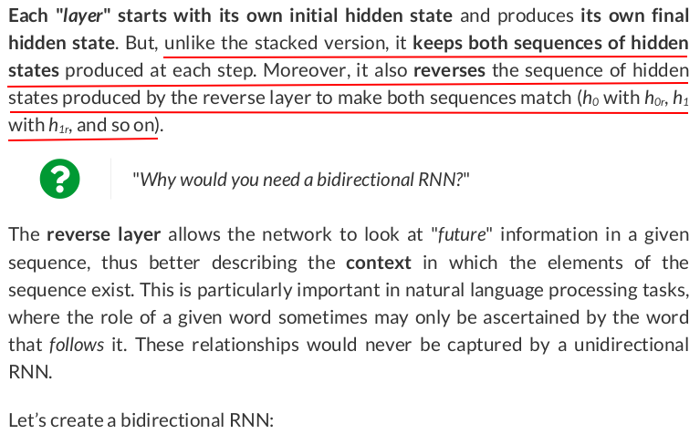
From its state dictionary, we can see it has two groups of weights and biases, one for each layer, with each layer indicated by its corresponding suffix (_l0 and _l0_reverse).
Once again, let’s create two simple RNNs, and then use the weights and biases above to set their weights accordingly. Each RNN will behave as one of the layers from the bidirectional one:
rnn_forward = nn.RNN(input_size=2, hidden_size=2, batch_first=True)
rnn_reverse = nn.RNN(input_size=2, hidden_size=2, batch_first=True)

state_list = list(state.items())
rnn_forward.load_state_dict(dict(state_list[:4]))
rnn_reverse.load_state_dict(dict([(k[:-8], v) for k, v in state_list[4:]]))

# <All keys matched successfully>

x_rev = torch.flip(x, dims=[1])  # N, L, F
x, x_rev
(tensor([[[ 1.1767, -0.8233],
          [-0.8233, -0.8233],
          [-0.8233,  1.1767],
          [ 1.1767,  1.1767]]]),
 tensor([[[ 1.1767,  1.1767],
          [-0.8233,  1.1767],
          [-0.8233, -0.8233],
          [ 1.1767, -0.8233]]]))

out, hidden = rnn_forward(x)
out_rev, hidden_rev = rnn_reverse(x_rev)
out_rev_back = torch.flip(out_rev, dims=[1])

out, out_rev_back, hidden, hidden_rev
(tensor([[[ 0.8533,  0.6675],
          [-0.6407, -0.7121],
          [-0.2594,  0.6654],
          [ 0.1636,  0.6967]]], grad_fn=<TransposeBackward1>),
 tensor([[[-0.4668,  0.2006],
          [ 0.8899,  0.0787],
          [ 0.1064, -0.8927],
          [-0.9374, -0.8478]]], grad_fn=<FlipBackward0>),
 tensor([[[0.1636, 0.6967]]], grad_fn=<StackBackward0>),
 tensor([[[-0.4668,  0.2006]]], grad_fn=<StackBackward0>))
torch.cat([out, out_rev_back], dim=2), torch.cat([hidden, hidden_rev])
(tensor([[[ 0.8533,  0.6675, -0.4668,  0.2006],
          [-0.6407, -0.7121,  0.8899,  0.0787],
          [-0.2594,  0.6654,  0.1064, -0.8927],
          [ 0.1636,  0.6967, -0.9374, -0.8478]]], grad_fn=<CatBackward0>),
 tensor([[[ 0.1636,  0.6967]],

         [[-0.4668,  0.2006]]], grad_fn=<CatBackward0>))
Done! We’ve replicated the inner workings of a bidirectional RNN using two simple RNNs. You can double-check the results by feeding the sequence of data points to the actual bidirectional RNN:
out, hidden = rnn_bidirect(x)
out, hidden
(tensor([[[ 0.8533,  0.6675, -0.4668,  0.2006],
          [-0.6407, -0.7121,  0.8899,  0.0787],
          [-0.2594,  0.6654,  0.1064, -0.8927],
          [ 0.1636,  0.6967, -0.9374, -0.8478]]], grad_fn=<TransposeBackward1>),
 tensor([[[ 0.1636,  0.6967]],

         [[-0.4668,  0.2006]]], grad_fn=<StackBackward0>))
And, once again, you’ll get the very same results.
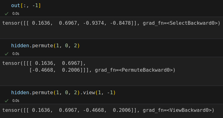

out[:, -1] == hidden.permute(1, 0, 2).view(1, -1)

# tensor([[ True,  True, False, False]])

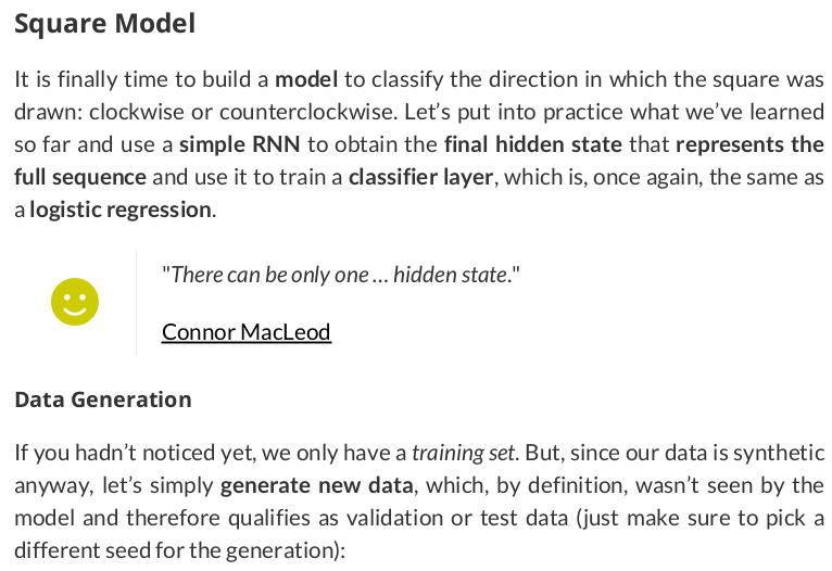
test_points, test_directions = generate_sequences(seed=19)

train_data = TensorDataset(torch.as_tensor(points).float(), torch.as_tensor(directions).view(-1, 1).float())
test_data = TensorDataset(torch.as_tensor(test_points).float(), torch.as_tensor(test_directions).view(-1, 1).float())

train_loader = DataLoader(dataset=train_data, batch_size=16, shuffle=True)
test_loader = DataLoader(dataset=test_data, batch_size=16)

class SquareModel(nn.Module):
    def __init__(self, n_inputs, hidden_size, n_outputs):
        super(SquareModel, self).__init__()
        self.n_inputs = n_inputs
        self.hidden_size = hidden_size
        self.n_outputs = n_outputs
        self.hidden = None
        # Simple RNN
        self.basic_rnn = nn.RNN(input_size=self.n_inputs, hidden_size=self.hidden_size, batch_first=True)
        # Classifier to produce as many logits as outputs
        self.classifier = nn.Linear(self.hidden_size, self.n_outputs)

    def forward(self, x):
        # x is batch first (N, L, F)
        # output is (N, L, H)
        # final hidden state is (1, N, H)
        batch_first_output, self.hidden = self.basic_rnn(x)

        # only last item in sequence (N, 1, H)
        last_output = batch_first_output[:, -1]
        # classifier will output (N, 1, n_outputs)
        out = self.classifier(last_output)

        # final output is (N, n_outputs)
        return out.view(-1, self.n_outputs)


torch.manual_seed(21)
model = SquareModel(n_inputs=2, hidden_size=2, n_outputs=1)
loss_fn = nn.BCEWithLogitsLoss()
optimizer = optim.Adam(model.parameters(), lr=0.01)

sbs_rnn = StepByStep(model, loss_fn, optimizer)
sbs_rnn.set_loaders(train_loader, test_loader)
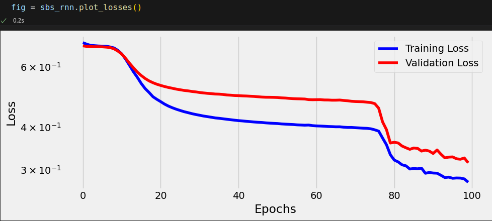
sbs_rnn.train(100)
StepByStep.loader_apply(test_loader, sbs_rnn.correct)
tensor([[56, 57],
        [50, 71]])
Our simple model hit 82.81% accuracy on the test data. Not bad, but, then again, this is a toy dataset.
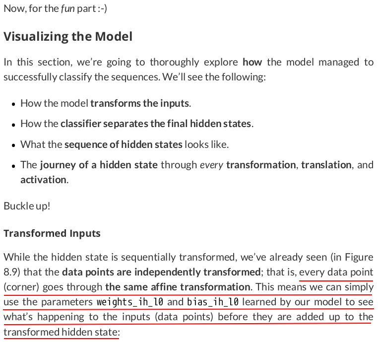
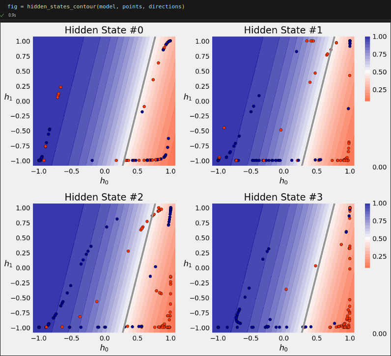
state = model.basic_rnn.state_dict()
state['weight_ih_l0'], state['bias_ih_l0']
(tensor([[-0.4448, -1.8874],
         [-2.4196, -1.9840]], device='cuda:0'),
 tensor([0.0324, 0.0598], device='cuda:0'))


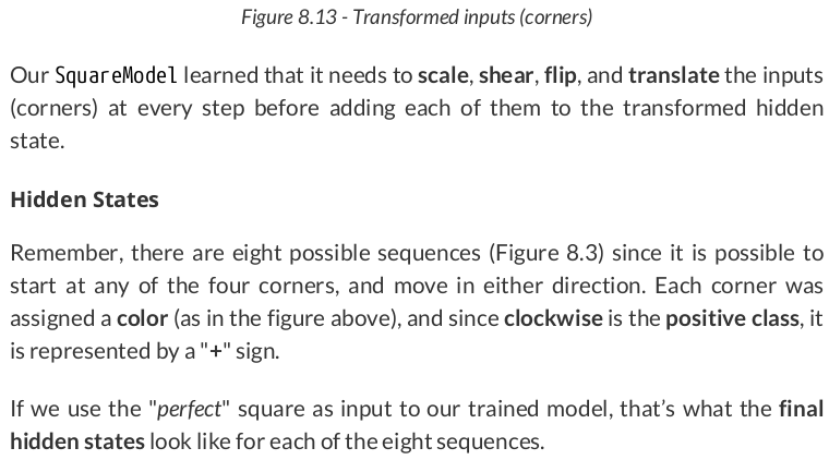
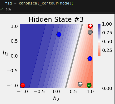
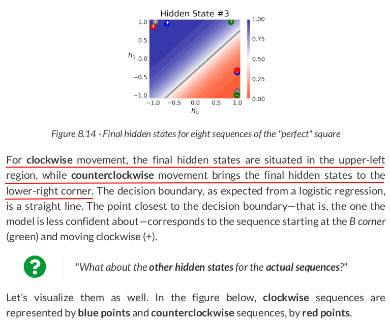

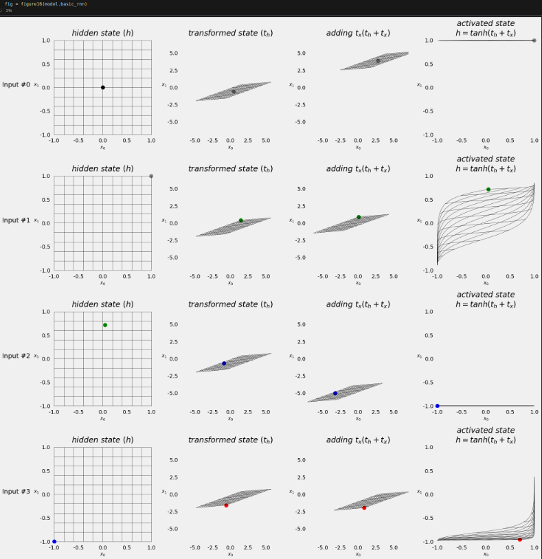
square = torch.tensor([[-1, -1], [-1, 1], [1, 1], [1, -1]]).float().view(1, 4, 2)
model(square.to(sbs_rnn.device))
model.hidden

# tensor([[[ 0.6983, -0.9612]]], device='cuda:0', grad_fn=<CudnnRnnBackward0>)
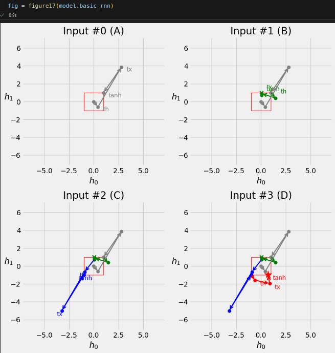
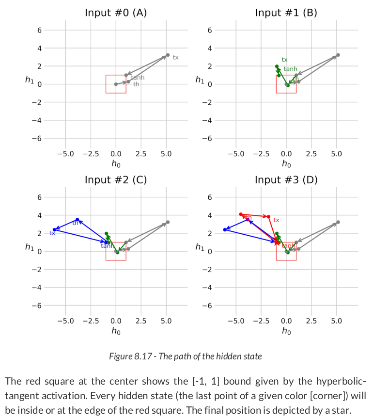


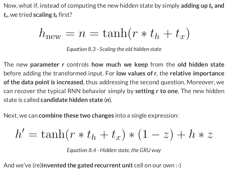
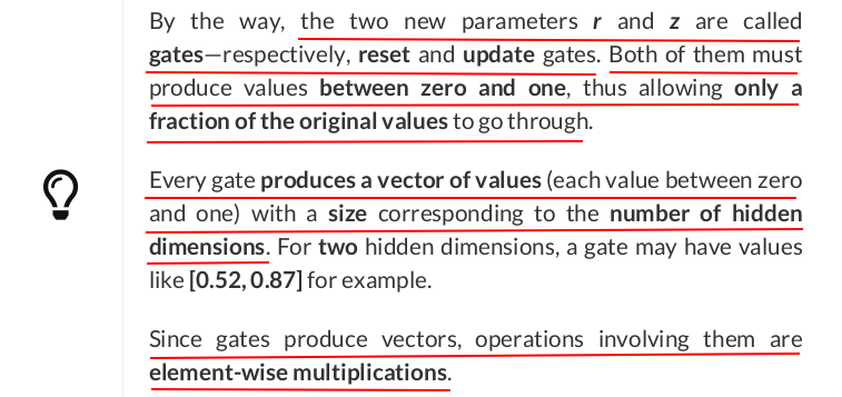
n_features = 2
hidden_dim = 2

torch.manual_seed(17)
gru_cell = nn.GRUCell(input_size=n_features, hidden_size=hidden_dim)
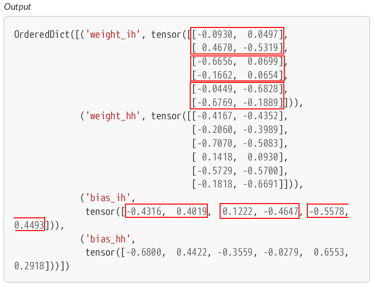
gru_state = gru_cell.state_dict()
gru_state
OrderedDict([('weight_ih',
              tensor([[-0.0930,  0.0497],
                      [ 0.4670, -0.5319],
                      [-0.6656,  0.0699],
                      [-0.1662,  0.0654],
                      [-0.0449, -0.6828],
                      [-0.6769, -0.1889]])),
             ('weight_hh',
              tensor([[-0.4167, -0.4352],
                      [-0.2060, -0.3989],
                      [-0.7070, -0.5083],
                      [ 0.1418,  0.0930],
                      [-0.5729, -0.5700],
                      [-0.1818, -0.6691]])),
             ('bias_ih',
              tensor([-0.4316,  0.4019,  0.1222, -0.4647, -0.5578,  0.4493])),
             ('bias_hh',
              tensor([-0.6800,  0.4422, -0.3559, -0.0279,  0.6553,  0.2918]))])

Wx, bx = gru_state['weight_ih'], gru_state['bias_ih']
Wh, bh = gru_state['weight_hh'], gru_state['bias_hh']

print(Wx.shape, Wh.shape)
print(bx.shape, bh.shape)
torch.Size([6, 2]) torch.Size([6, 2])
torch.Size([6]) torch.Size([6])

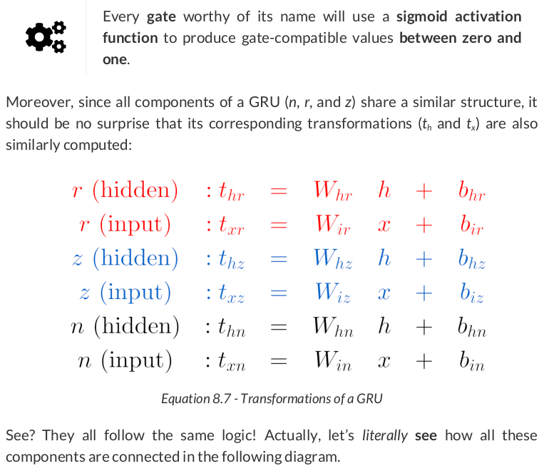
In code, we can use split() to get tensors for each of the components:
W_xr, W_xz, W_xn = Wx.split(hidden_dim, dim=0)
print(W_xr.numpy(), W_xz.numpy(), W_xn.numpy(), sep=',\n')

b_xr, b_xz, b_xn = bx.split(hidden_dim, dim=0)
print(b_xr.numpy(), b_xz.numpy(), b_xn.numpy(), sep=', ')

W_hr, W_hz, W_hn = Wh.split(hidden_dim, dim=0)
print(W_hr.numpy(), W_hz.numpy(), W_hn.numpy(), sep=',\n')

b_hr, b_hz, b_hn = bh.split(hidden_dim, dim=0)
print(b_hr.numpy(), b_hz.numpy(), b_hn.numpy(), sep=', ')
[[-0.09299693  0.04965244]
 [ 0.46698564 -0.53193724]],
[[-0.66564053  0.06985663]
 [-0.16618267  0.0654211 ]],
[[-0.04486127 -0.68284917]
 [-0.6768686  -0.1889009 ]]
[-0.43164796  0.40188766], [ 0.12215219 -0.46473247], [-0.5577969  0.4492511]
[[-0.4166978  -0.4352161 ]
 [-0.20599432 -0.3988804 ]],
[[-0.7069572  -0.5083179 ]
 [ 0.14182186  0.0930218 ]],
[[-0.57290494 -0.56999516]
 [-0.18181518 -0.6691437 ]]
[-0.6800008  0.4422237], [-0.35588545 -0.02794665], [0.655336  0.2917871]
Next, let’s use the weights and biases to create the corresponding linear layers:
def linear_layers(Wx, bx, Wh, bh):
    hidden_dim, n_features = Wx.size()
    lin_input = nn.Linear(n_features, hidden_dim)
    lin_input.load_state_dict({'weight': Wx, 'bias': bx})
    lin_hidden = nn.Linear(hidden_dim, hidden_dim)
    lin_hidden.load_state_dict({'weight': Wh, 'bias': bh})
    return lin_input, lin_hidden

r_input, r_hidden = linear_layers(W_xr, b_xr, W_hr, b_hr)  # reset gate - red
z_input, z_hidden = linear_layers(W_xz, b_xz, W_hz, b_hz)  # update gate - blue
n_input, n_hidden = linear_layers(W_xn, b_xn, W_hn, b_hn)  # candidate state - black
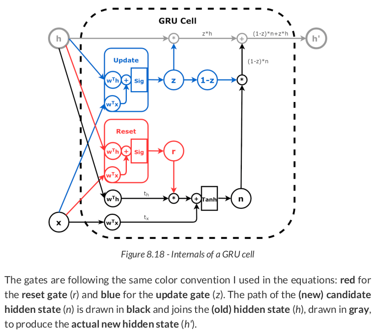
Then, let’s use these layers to create functions that replicate both gates (r and z) and the candidate hidden state (n):
def reset_gate(h, x):
    t_hr = r_hidden(h)
    t_xr = r_input(x)
    r = torch.sigmoid(t_hr + t_xr)
    return r  # red

def update_gate(h, x):
    t_hz = z_hidden(h)
    t_xz = z_input(x)
    z = torch.sigmoid(t_hz + t_xz)
    return z  # blue

def candidate_n(h, x, r):
    t_hn = n_hidden(h)
    t_xn = n_input(x)
    n = torch.tanh(r * t_hn + t_xn)
    return n  # black

initial_hidden = torch.zeros(1, hidden_dim)
x = torch.as_tensor(points[0]).float()
first_corner = x[0:1]
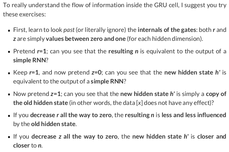
We use both values to get the output from the reset gate (r):
r = reset_gate(initial_hidden, first_corner)
r

# tensor([[0.2206, 0.8619]], grad_fn=<SigmoidBackward0>)

n = candidate_n(initial_hidden, first_corner, r)
n

# tensor([[0.0959, 0.0598]], grad_fn=<TanhBackward0>)
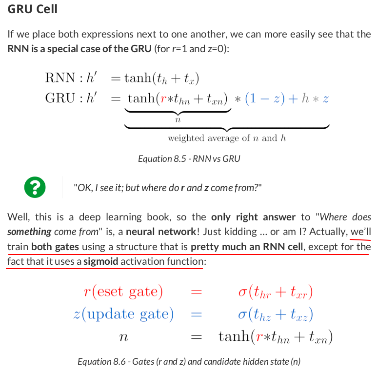
That would be the end of it, and that would be the new hidden state if it wasn’t for the update gate (z):
z = update_gate(initial_hidden, first_corner)
z

# tensor([[0.2545, 0.3225]], grad_fn=<SigmoidBackward0>)
Another short pause here—the update gate is telling us to keep 25.45% of the first and 32.25% of the second dimensions of the initial hidden state. The remaining 74.55% and 67.75%, respectively, are coming from the candidate hidden state (n). So, the new hidden state (h_prime) is computed accordingly:
h_prime = n * (1 - z) + initial_hidden * z
h_prime

# tensor([[0.0715, 0.0405]], grad_fn=<AddBackward0>)
Now, let’s take a quick sanity check, feeding the same input to the original GRU cell:
gru_cell(first_corner)

# tensor([[0.0715, 0.0405]], grad_fn=<AddBackward0>)
Perfect match!
But, then again, you’re likely not inclined to loop over the sequence yourself while using a GRU cell, right? You probably want to use a full-fledged…

class SquareModelGRU(nn.Module):
    def __init__(self, n_inputs, hidden_size, n_outputs):
        super(SquareModelGRU, self).__init__()
        self.n_inputs = n_inputs
        self.hidden_size = hidden_size
        self.n_outputs = n_outputs
        self.hidden = None
        # Simple GRU
        self.basic_rnn = nn.GRU(self.n_inputs, self.hidden_size, batch_first=True)
        # Classifier to produce as many logits as outputs
        self.classifier = nn.Linear(self.hidden_size, self.n_outputs)

    def forward(self, x):
        # x is batch first (N, L, F)
        # output is (N, L, H)
        # final hidden state is (1, N, H)
        batch_first_output, self.hidden = self.basic_rnn(x)

        # only last item in sequence (N, 1, H)
        last_output = batch_first_output[:, -1]
        # classifier will output (N, 1, n_outputs)
        out = self.classifier(last_output)

        # final output is (N, n_outputs)
        return out.view(-1, self.n_outputs)


torch.manual_seed(21)
model = SquareModelGRU(n_inputs=2, hidden_size=2, n_outputs=1)
loss_fn = nn.BCEWithLogitsLoss()
optimizer = optim.Adam(model.parameters(), lr=0.01)

sbs_gru = StepByStep(model, loss_fn, optimizer)
sbs_gru.set_loaders(train_loader, test_loader)
sbs_gru.train(100)

Cool—the loss decreased much quicker now, and all it takes is switching from RNN to GRU.
StepByStep.loader_apply(test_loader, sbs_gru.correct)
tensor([[57, 57],
        [71, 71]])
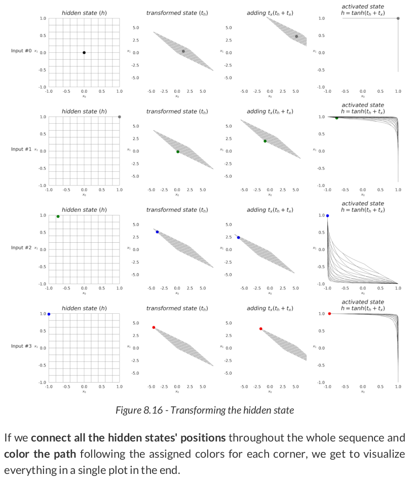
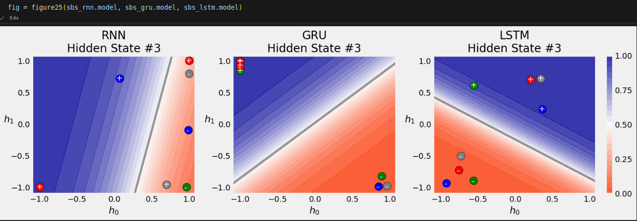
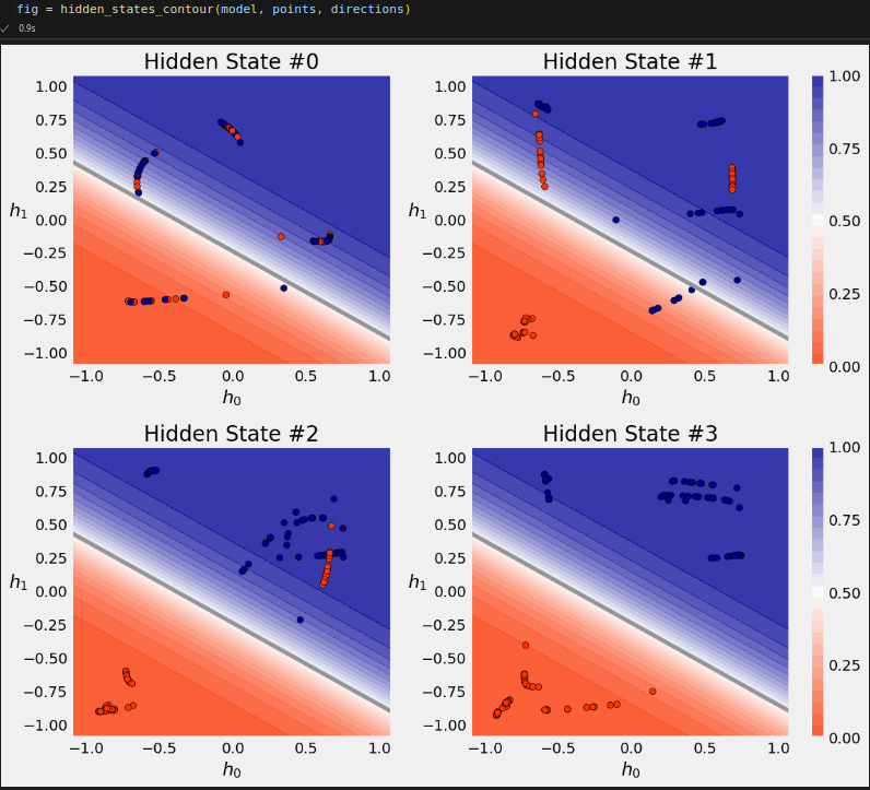
That’s 100% accuracy! Let’s try to visualize the effect of the GRU architecture on the classification of the hidden states.

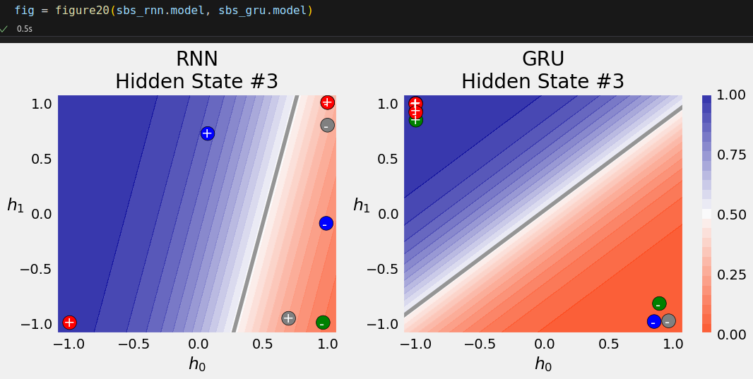
The GRU model achieves a better separation of the sequences than its RNN counterpart. What about the actual sequences?
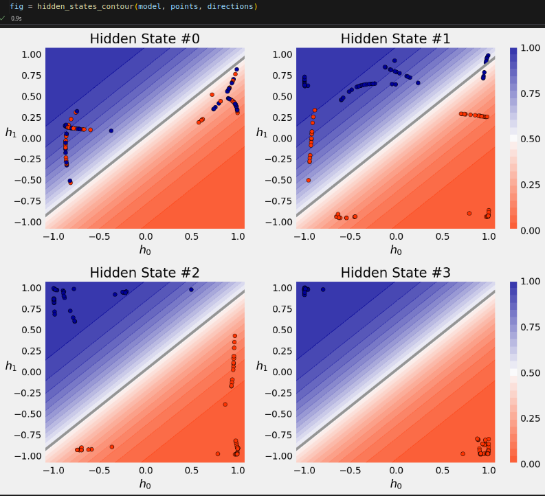
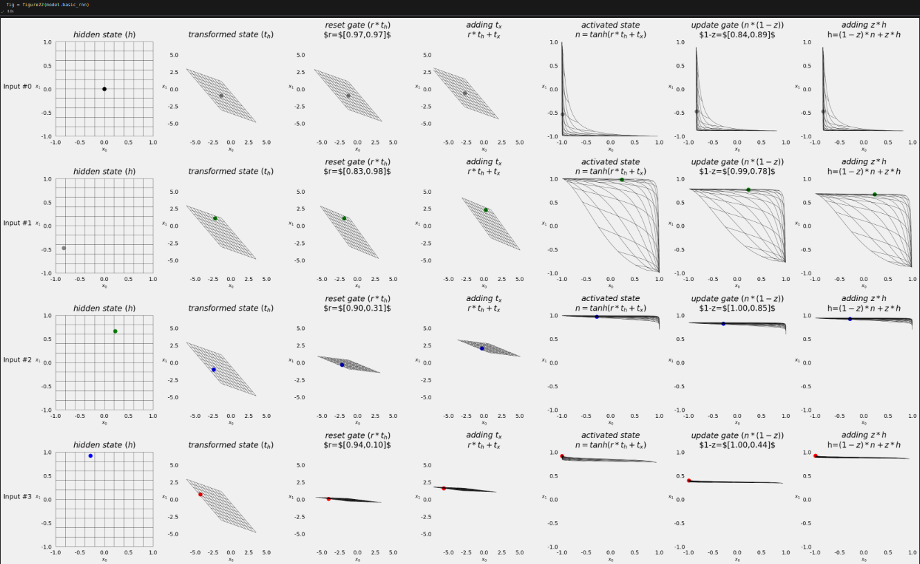
Figure 8.22 - Transforming the hidden state


n_features = 2
hidden_dim = 2

torch.manual_seed(17)
lstm_cell = nn.LSTMCell(input_size=n_features, hidden_size=hidden_dim)
lstm_state = lstm_cell.state_dict()
lstm_state
OrderedDict([('weight_ih',
              tensor([[-0.0930,  0.0497],
                      [ 0.4670, -0.5319],
                      [-0.6656,  0.0699],
                      [-0.1662,  0.0654],
                      [-0.0449, -0.6828],
                      [-0.6769, -0.1889],
                      [-0.4167, -0.4352],
                      [-0.2060, -0.3989]])),
             ('weight_hh',
              tensor([[-0.7070, -0.5083],
                      [ 0.1418,  0.0930],
                      [-0.5729, -0.5700],
                      [-0.1818, -0.6691],
                      [-0.4316,  0.4019],
                      [ 0.1222, -0.4647],
                      [-0.5578,  0.4493],
                      [-0.6800,  0.4422]])),
             ('bias_ih',
              tensor([-0.3559, -0.0279,  0.6553,  0.2918,  0.4007,  0.3262, -0.0778, -0.3002])),
             ('bias_hh',
              tensor([-0.3991, -0.3200,  0.3483, -0.2604, -0.1582,  0.5558,  0.5761, -0.3919]))])

Wx, bx = lstm_state['weight_ih'], lstm_state['bias_ih']
Wh, bh = lstm_state['weight_hh'], lstm_state['bias_hh']

# Split weights and biases for data points
W_xi, W_xf, W_xg, W_xo = Wx.split(hidden_dim, dim=0)
b_xi, b_xf, b_xg, b_xo = bx.split(hidden_dim, dim=0)

# Split weights and biases for hidden state
W_hi, W_hf, W_hg, W_ho = Wh.split(hidden_dim, dim=0)
b_hi, b_hf, b_hg, b_ho = bh.split(hidden_dim, dim=0)

# Create linear layers for the components
i_input, i_hidden = linear_layers(W_xi, b_xi, W_hi, b_hi)  # input gate - green
f_input, f_hidden = linear_layers(W_xf, b_xf, W_hf, b_hf)  # forget gate - red
o_input, o_hidden = linear_layers(W_xo, b_xo, W_ho, b_ho)  # output gate - blue

g_cell = nn.RNNCell(n_features, hidden_dim)  # black
g_cell.load_state_dict({'weight_ih': W_xg, 'bias_ih': b_xg,
                        'weight_hh': W_hg, 'bias_hh': b_hg})

# <All keys matched successfully>
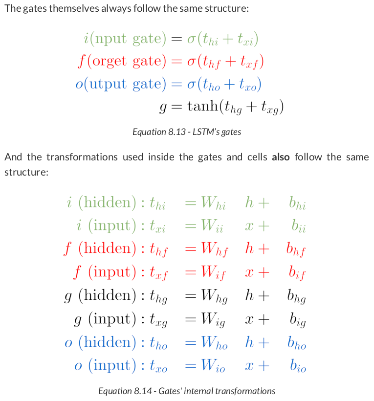
That was easy, right? Since the other components are gates, we need to create functions for them:
def forget_gate(h, x):
    t_hf = f_hidden(h)
    t_xf = f_input(x)
    f = torch.sigmoid(t_hf + t_xf)
    return f  # red

def output_gate(h, x):
    t_ho = o_hidden(h)
    t_xo = o_input(x)
    o = torch.sigmoid(t_ho + t_xo)
    return o  # blue

def input_gate(h, x):
    t_hi = i_hidden(h)
    t_xi = i_input(x)
    i = torch.sigmoid(t_hi + t_xi)
    return i  # green

initial_hidden = torch.zeros(1, hidden_dim)
initial_cell = torch.zeros(1, hidden_dim)

x = torch.as_tensor(points[0]).float()
first_corner = x[0:1]
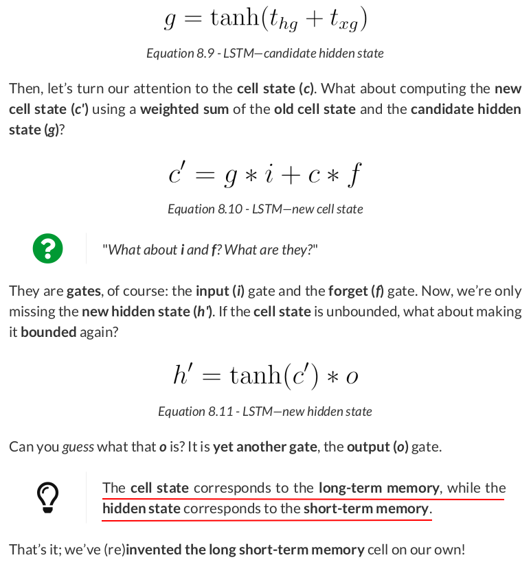
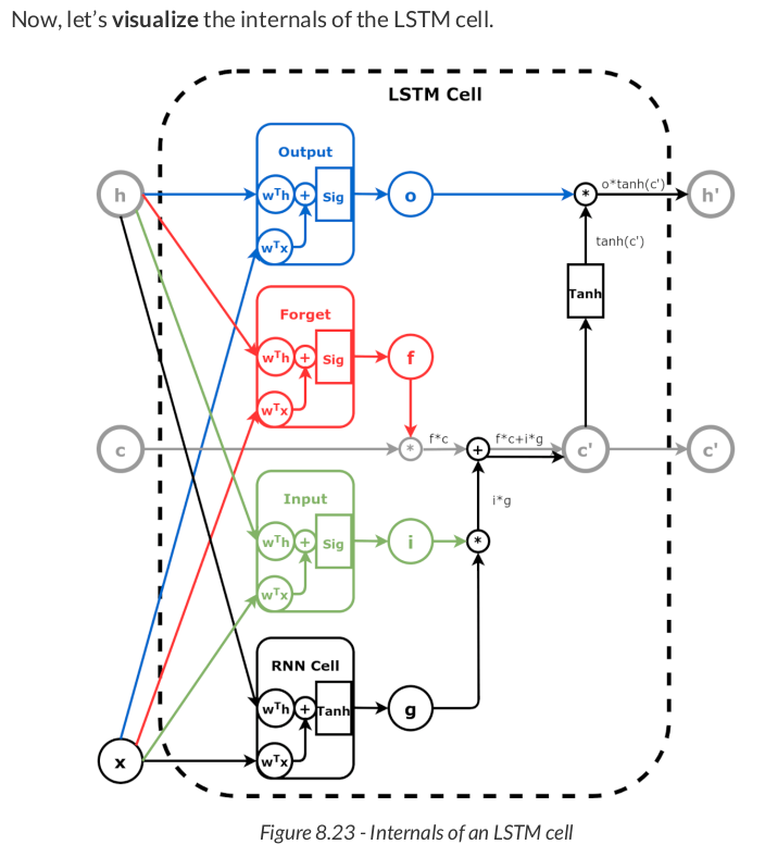
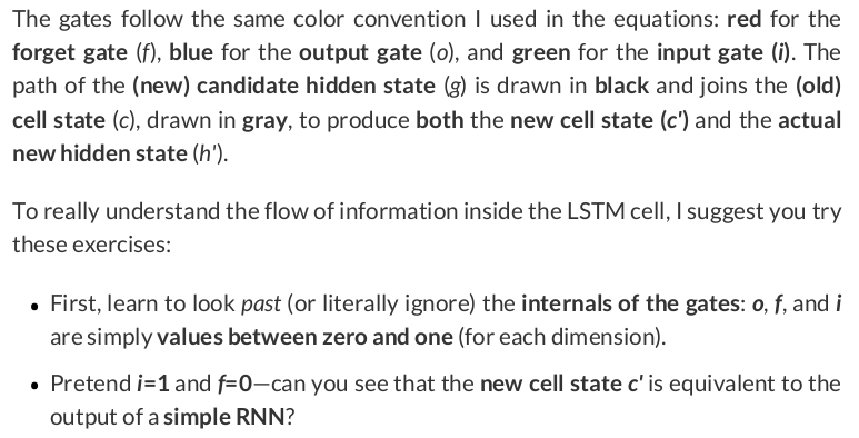
Then, we start by computing the gated input using both the RNN cell (g) and its corresponding gate (i):
g = g_cell(first_corner)
i = input_gate(initial_hidden, first_corner)
gated_input = g * i
gated_input

# tensor([[0.1832, 0.1548]], grad_fn=<MulBackward0>)
Next, we compute the gated cell state using the old cell state (c) and its corresponding gate, the forget (f) gate:
f = forget_gate(initial_hidden, first_corner)
gated_cell = initial_cell * f
gated_cell

# tensor([[0., 0.]], grad_fn=<MulBackward0>)

c_prime = gated_cell + gated_input
c_prime

# tensor([[0.1832, 0.1548]], grad_fn=<AddBackward0>)
The only thing missing is "converting" the cell state to a new hidden state (h') using the hyperbolic tangent and the output (o) gate:
o = output_gate(initial_hidden, first_corner)
h_prime = o * torch.tanh(c_prime)
h_prime

# tensor([[0.1070, 0.0542]], grad_fn=<MulBackward0>)
The LSTM cell must return both states, hidden and cell, in that order, as a tuple:
(h_prime, c_prime)
(tensor([[0.1070, 0.0542]], grad_fn=<MulBackward0>),
 tensor([[0.1832, 0.1548]], grad_fn=<AddBackward0>))

lstm_cell(first_corner)
(tensor([[0.1070, 0.0542]], grad_fn=<MulBackward0>),
 tensor([[0.1832, 0.1548]], grad_fn=<AddBackward0>))
class SquareModelLSTM(nn.Module):
    def __init__(self, n_inputs, hidden_dim, n_outputs):
        super(SquareModelLSTM, self).__init__()
        self.n_inputs = n_inputs
        self.hidden_dim = hidden_dim
        self.n_outputs = n_outputs
        self.hidden = None
        self.cell = None
        # Simple LSTM
        self.basic_rnn = nn.LSTM(self.n_inputs, self.hidden_dim, batch_first=True)
        # Classifier to produce as many logits as outputs
        self.classifier = nn.Linear(self.hidden_dim, self.n_outputs)

    def forward(self, X):
        # X is batch first (N, L, F)
        # output is (N, L, H)
        # final hidden state is (1, N, H)
        # final cell state is (1, N, H)
        batch_first_output, (self.hidden, self.cell) = self.basic_rnn(X)

        # only last item in sequence (N, 1, H)
        last_output = batch_first_output[:, -1]
        # classifier will output (N, 1, n_outputs)
        out = self.classifier(last_output)

        # final output is (N, n_outputs)
        return out.view(-1, self.n_outputs)

torch.manual_seed(21)
model = SquareModelLSTM(n_inputs=2, hidden_dim=2, n_outputs=1)
loss_fn = nn.BCEWithLogitsLoss()
optimizer = optim.Adam(model.parameters(), lr=0.01)

sbs_lstm = StepByStep(model, loss_fn, optimizer)
sbs_lstm.set_loaders(train_loader, test_loader)
sbs_lstm.train(100)

StepByStep.loader_apply(test_loader, sbs_lstm.correct)
tensor([[57, 57],
        [71, 71]])
And that’s 100% accuracy again!



s0 = points[0]      # 4 data points
s1 = points[1][2:]  # 2 data points
s2 = points[2][1:]  # 3 data points

s0.shape, s1.shape, s2.shape

# ((4, 2), (2, 2), (3, 2))

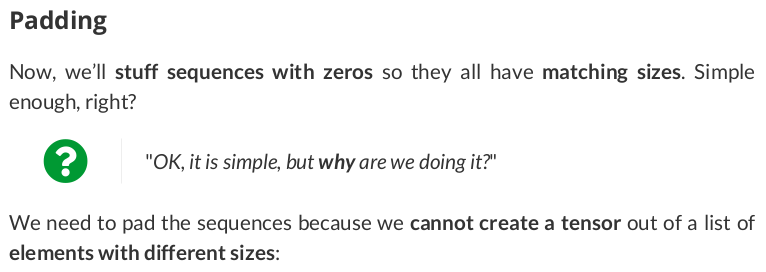


from torch.nn.utils import rnn as rnn_utils

seq_tensors = [torch.as_tensor(seq).float() for seq in all_seqs]
padded = rnn_utils.pad_sequence(seq_tensors, batch_first=True)
padded
tensor([[[ 1.1767, -0.8233],
         [-0.8233, -0.8233],
         [-0.8233,  1.1767],
         [ 1.1767,  1.1767]],

        [[-0.3331,  1.6669],
         [ 1.6669,  1.6669],
         [ 0.0000,  0.0000],
         [ 0.0000,  0.0000]],

        [[-0.6587,  1.3413],
         [-0.6587, -0.6587],
         [ 1.3413, -0.6587],
         [ 0.0000,  0.0000]]])
Both the second and the third sequences were shorter than the first, so they got padded accordingly to match the length of the longest sequence.
Now we can proceed as usual and feed the padded sequences to an RNN and look at the results:
torch.manual_seed(11)
rnn = nn.RNN(2, 2, batch_first=True)

output_padded, hidden_padded = rnn(padded)
output_padded
tensor([[[-0.6599,  0.9755],
         [ 0.3704,  0.2268],
         [ 0.2619, -0.1903],
         [-0.6919,  0.8826]],

        [[-0.0903, -0.0102],
         [-0.7993,  0.8760],
         [-0.0791,  0.4186],
         [-0.1184,  0.6475]],

        [[ 0.0771, -0.0810],
         [ 0.1019,  0.7203],
         [-0.5837,  0.9530],
         [-0.0326,  0.4061]]], grad_fn=<TransposeBackward1>)
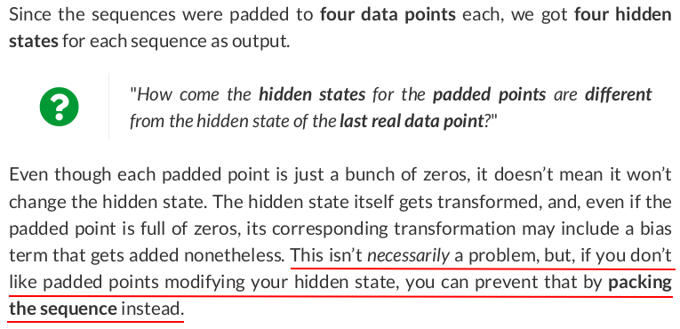
Before moving on to packed sequences, though, let’s just check the (permuted, batch-first) final hidden state:
hidden_padded.permute(1, 0, 2)
tensor([[[-0.6919,  0.8826]],

        [[-0.1184,  0.6475]],

        [[-0.0326,  0.4061]]], grad_fn=<PermuteBackward0>)

packed = rnn_utils.pack_sequence(seq_tensors, enforce_sorted=False)
packed
PackedSequence(data=tensor([[ 1.1767, -0.8233],
        [-0.6587,  1.3413],
        [-0.3331,  1.6669],
        [-0.8233, -0.8233],
        [-0.6587, -0.6587],
        [ 1.6669,  1.6669],
        [-0.8233,  1.1767],
        [ 1.3413, -0.6587],
        [ 1.1767,  1.1767]]), batch_sizes=tensor([3, 3, 2, 1]), sorted_indices=tensor([0, 2, 1]), unsorted_indices=tensor([0, 2, 1]))
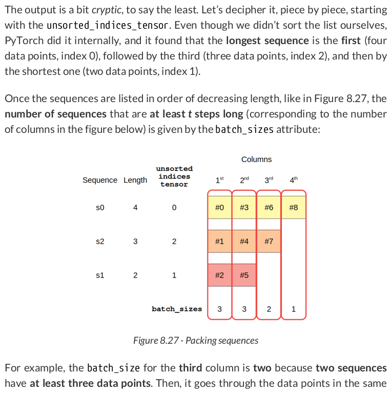
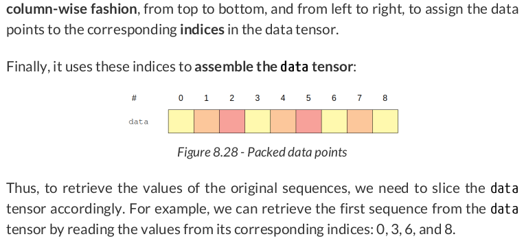
(packed.data[[0, 3, 6, 8]] == seq_tensors[0]).all()

# tensor(True)
Once the sequence is properly packed, we can feed it directly to an RNN:
output_packed, hidden_packed = rnn(packed)
output_packed, hidden_packed
(PackedSequence(data=tensor([[-0.6599,  0.9755],
         [ 0.0771, -0.0810],
         [-0.0903, -0.0102],
         [ 0.3704,  0.2268],
         [ 0.1019,  0.7203],
         [-0.7993,  0.8760],
         [ 0.2619, -0.1903],
         [-0.5837,  0.9530],
         [-0.6919,  0.8826]], grad_fn=<CatBackward0>), batch_sizes=tensor([3, 3, 2, 1]), sorted_indices=tensor([0, 2, 1]), unsorted_indices=tensor([0, 2, 1])),
 tensor([[[-0.6919,  0.8826],
          [-0.7993,  0.8760],
          [-0.5837,  0.9530]]], grad_fn=<IndexSelectBackward0>))

hidden_packed == hidden_padded
tensor([[[ True,  True],
         [False, False],
         [False, False]]])
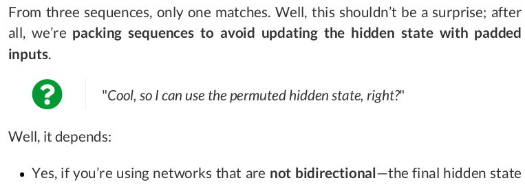

output_packed.data[[2, 5]] # x1 sequence
tensor([[-0.0903, -0.0102],
        [-0.7993,  0.8760]], grad_fn=<IndexBackward0>)

output_unpacked, seq_sizes = rnn_utils.pad_packed_sequence(output_packed, batch_first=True)
output_unpacked, seq_sizes
(tensor([[[-0.6599,  0.9755],
          [ 0.3704,  0.2268],
          [ 0.2619, -0.1903],
          [-0.6919,  0.8826]],

         [[-0.0903, -0.0102],
          [-0.7993,  0.8760],
          [ 0.0000,  0.0000],
          [ 0.0000,  0.0000]],

         [[ 0.0771, -0.0810],
          [ 0.1019,  0.7203],
          [-0.5837,  0.9530],
          [ 0.0000,  0.0000]]], grad_fn=<IndexSelectBackward0>),
 tensor([4, 2, 3]))

output_unpacked[:, -1]
tensor([[-0.6919,  0.8826],
        [ 0.0000,  0.0000],
        [ 0.0000,  0.0000]], grad_fn=<SelectBackward0>)
So, to actually get the last output, we need to use some fancy indexing and the information about original sizes returned by pad_packed_sequence():
seq_idx = torch.arange(seq_sizes.size(0))
output_unpacked[seq_idx, seq_sizes-1]
tensor([[-0.6919,  0.8826],
        [-0.7993,  0.8760],
        [-0.5837,  0.9530]], grad_fn=<IndexBackward0>)

len_seqs = [len(seq) for seq in all_seqs]
len_seqs

# [4, 2, 3]
And then pass them as an argument:
packed = rnn_utils.pack_padded_sequence(padded, len_seqs, enforce_sorted=False, batch_first=True)
packed
PackedSequence(data=tensor([[ 1.1767, -0.8233],
        [-0.6587,  1.3413],
        [-0.3331,  1.6669],
        [-0.8233, -0.8233],
        [-0.6587, -0.6587],
        [ 1.6669,  1.6669],
        [-0.8233,  1.1767],
        [ 1.3413, -0.6587],
        [ 1.1767,  1.1767]]), batch_sizes=tensor([3, 3, 2, 1]), sorted_indices=tensor([0, 2, 1]), unsorted_indices=tensor([0, 2, 1]))

var_points, var_directions = generate_sequences(variable_len=True)
var_points[:2]
[array([[ 1.73270012, -0.26729988],
        [-0.26729988, -0.26729988],
        [-0.26729988,  1.73270012],
        [ 1.73270012,  1.73270012]]),
 array([[ 1.44822753, -0.55177247],
        [-0.55177247, -0.55177247],
        [-0.55177247,  1.44822753],
        [ 1.44822753,  1.44822753]])]

class CustomDataset(Dataset):
    def __init__(self, x, y):
        self.x = [torch.as_tensor(s).float() for s in x]
        self.y = torch.as_tensor(y).float().view(-1, 1)

    def __getitem__(self, index):
        return (self.x[index], self.y[index])

    def __len__(self):
        return len(self.x)

train_var_data = CustomDataset(var_points, var_directions)
But this is not enough; if we create a data loader for our custom dataset and try to retrieve a mini-batch out of it, it will raise an error:
train_var_loader = DataLoader(train_var_data, batch_size=16, shuffle=True)
next(iter(train_var_loader))
RuntimeError: stack expects each tensor to be equal size, but got [3, 2] at entry 0 and [2, 2] at entry 1

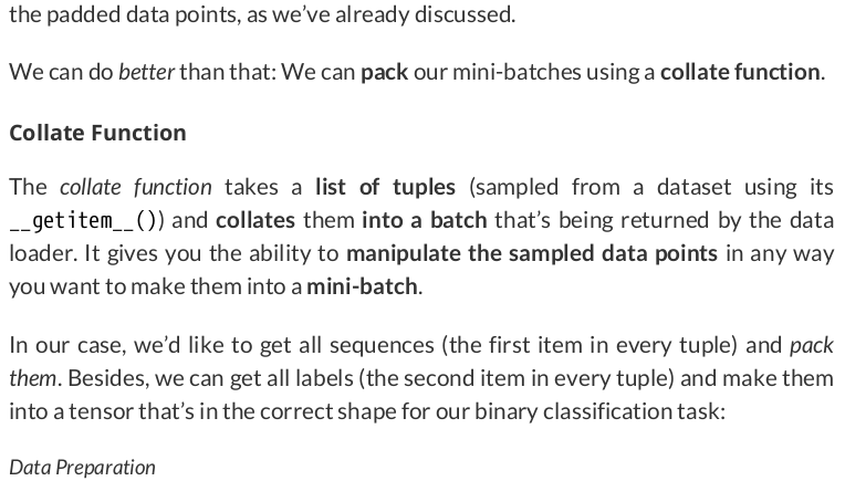
def pack_collate(batch):
    X = [item[0] for item in batch]
    y = [item[1] for item in batch]
    X_pack = rnn_utils.pack_sequence(X, enforce_sorted=False)

    return X_pack, torch.as_tensor(y).view(-1, 1)
Let’s see the function in action by creating a dummy batch of two elements and applying the function to it:
# list of tuples returned by the dataset
dummy_batch = [train_var_data[0], train_var_data[1]]
dummy_x, dummy_y = pack_collate(dummy_batch)
dummy_x
PackedSequence(data=tensor([[ 1.7327, -0.2673],
        [ 1.4482, -0.5518],
        [-0.2673, -0.2673],
        [-0.5518, -0.5518],
        [-0.2673,  1.7327],
        [-0.5518,  1.4482],
        [ 1.7327,  1.7327],
        [ 1.4482,  1.4482]]), batch_sizes=tensor([2, 2, 2, 2]), sorted_indices=tensor([0, 1]), unsorted_indices=tensor([0, 1]))
Two sequences of different sizes go in, one packed sequence comes out. Now we can create a data loader that uses our collate function:
Data Preparation
train_var_loader = DataLoader(train_var_data, batch_size=16, shuffle=True, collate_fn=pack_collate)
x_batch, y_batch = next(iter(train_var_loader))

class SquareModelPacked(nn.Module):
    def __init__(self, n_features, hidden_dim, n_outputs):
        super(SquareModelPacked, self).__init__()
        self.hidden_dim = hidden_dim
        self.n_features = n_features
        self.n_outputs = n_outputs
        self.hidden = None
        self.cell = None
        # Simple LSTM
        self.basic_rnn = nn.LSTM(self.n_features, self.hidden_dim, bidirectional=True)
        # Classifier to produce as many logits as outputs
        self.classifier = nn.Linear(2 * self.hidden_dim, self.n_outputs)

    def forward(self, X):
        # X is a PACKED sequence now

        # output is PACKED
        # final hidden state is (2, N, H) - bidirectional
        # final cell state is (2, N, H) - bidirectional
        rnn_out, (self.hidden, self.cell) = self.basic_rnn(X)
        # unpack the output (N, L, 2*H)
        batch_first_output, seq_sizes = rnn_utils.pad_packed_sequence(rnn_out, batch_first=True)

        # only last item in sequence (N, 1, 2*H)
        seq_idx = torch.arange(seq_sizes.size(0))
        last_output = batch_first_output[seq_idx, seq_sizes-1]
        # classifier will output (N, 1, n_outputs)
        out = self.classifier(last_output)

        # final output is (N, n_outputs)
        return out.view(-1, self.n_outputs)

torch.manual_seed(21)
model = SquareModelPacked(n_features=2, hidden_dim=2, n_outputs=1)
loss_fn = nn.BCEWithLogitsLoss()
optimizer = optim.Adam(model.parameters(), lr=0.01)

sbs_packed = StepByStep(model, loss_fn, optimizer)
sbs_packed.set_loaders(train_var_loader)
sbs_packed.train(100)
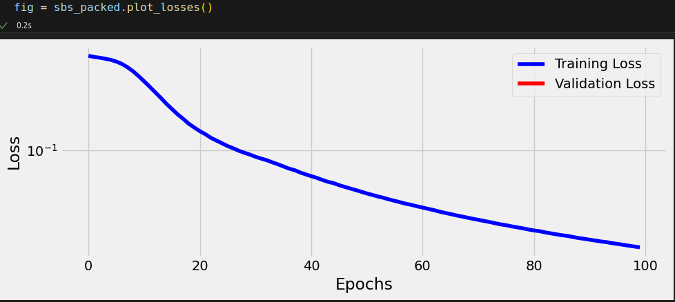
StepByStep.loader_apply(train_var_loader, sbs_packed.correct)
tensor([[65, 65],
        [63, 63]])
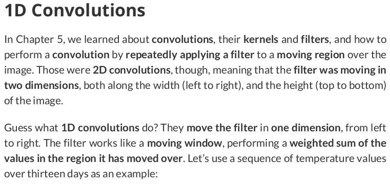
temperatures = np.array([5, 11, 15, 6, 5, 3, 3, 0, 0, 3, 4, 2, 1])

import torch.nn.functional as F

size = 5
weight = torch.ones(size) * 0.2
F.conv1d(torch.as_tensor(temperatures).float().view(1, 1, -1), weight=weight.view(1, 1, -1))
tensor([[[8.4000, 8.0000, 6.4000, 3.4000, 2.2000, 1.8000, 2.0000, 1.8000,
          2.0000]]])
seqs = torch.as_tensor(points).float() # N, L, F
seqs_length_last = seqs.permute(0, 2, 1)
seqs_length_last.shape # N, F=C, L

# torch.Size([128, 2, 4])

torch.manual_seed(17)
conv_seq = nn.Conv1d(in_channels=2, out_channels=1, kernel_size=2, bias=False)
conv_seq.weight, conv_seq.weight.shape
(Parameter containing:
 tensor([[[-0.0658,  0.0351],
          [ 0.3302, -0.3761]]], requires_grad=True),
 torch.Size([1, 2, 2]))
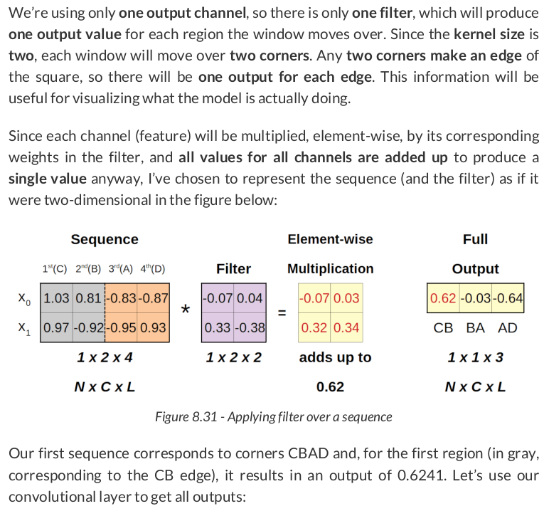
conv_seq(seqs_length_last[0:1])

# tensor([[[-0.0685, -0.6892,  0.0414]]], grad_fn=<ConvolutionBackward0>)
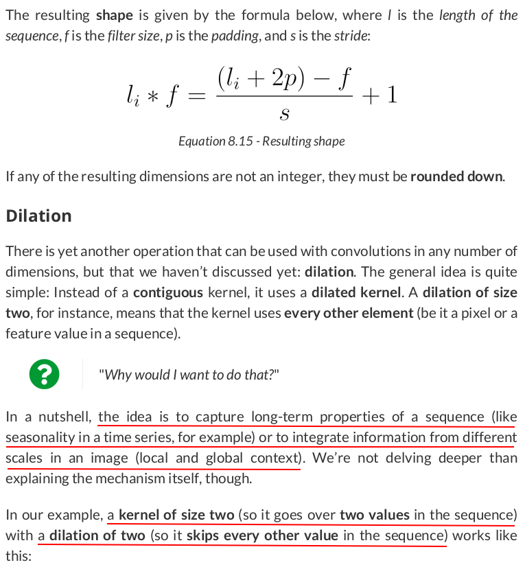
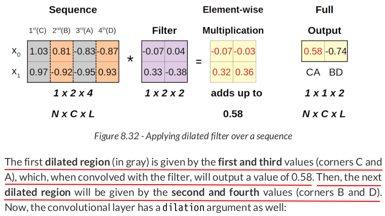
torch.manual_seed(17)
conv_dilated = nn.Conv1d(in_channels=2, out_channels=1, kernel_size=2, dilation=2, bias=False)
conv_dilated.weight, conv_dilated.weight.shape
(Parameter containing:
 tensor([[[-0.0658,  0.0351],
          [ 0.3302, -0.3761]]], requires_grad=True),
 torch.Size([1, 2, 2]))
conv_dilated(seqs_length_last[0:1])

# tensor([[[-0.8207, -0.6190]]], grad_fn=<ConvolutionBackward0>)
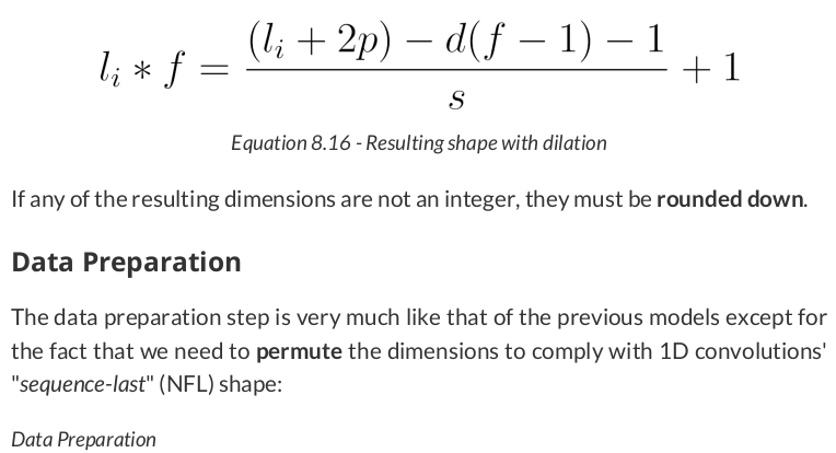
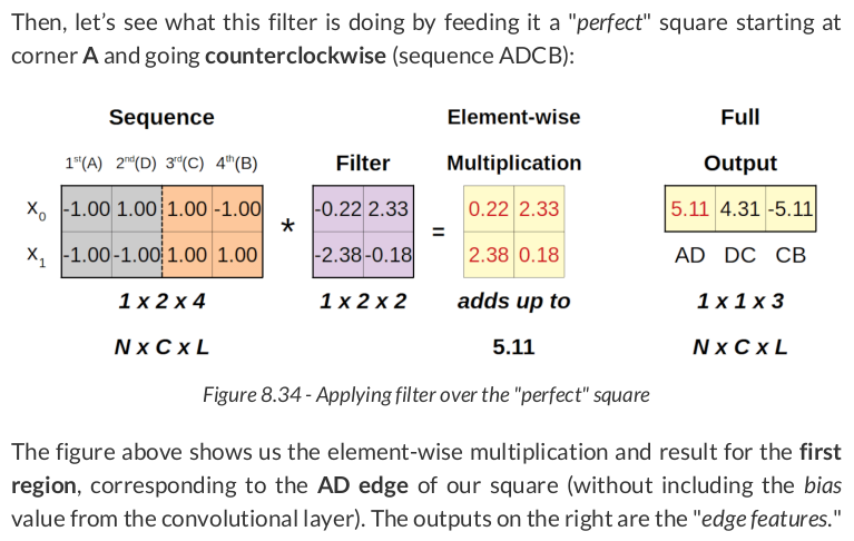
This output is smaller than the previous one because the dilation affects the shape of the output according to the formula below (d stands for dilation size):
train_data = TensorDataset(torch.as_tensor(points).float().permute(0, 2, 1),
                           torch.as_tensor(directions).view(-1, 1).float())
test_data = TensorDataset(torch.as_tensor(test_points).float().permute(0, 2, 1),
                          torch.as_tensor(test_directions).view(-1, 1).float())

train_loader = DataLoader(train_data, batch_size=16, shuffle=True)
test_loader = DataLoader(test_data, batch_size=16)

torch.manual_seed(21)
model = nn.Sequential()
model.add_module('conv1d', nn.Conv1d(2, 1, kernel_size=2))
model.add_module('relu', nn.ReLU())
model.add_module('flatten', nn.Flatten())
model.add_module('output', nn.Linear(3, 1))
loss_fn = nn.BCEWithLogitsLoss()
optimizer = optim.Adam(model.parameters(), lr=0.01)

sbs_conv1 = StepByStep(model, loss_fn, optimizer)
sbs_conv1.set_loaders(train_loader, test_loader)
sbs_conv1.train(100)
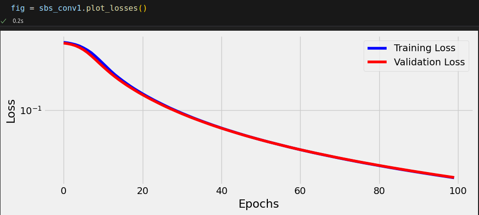
StepByStep.loader_apply(test_loader, sbs_conv1.correct)
tensor([[57, 57],
        [71, 71]])

model.conv1d.state_dict()
OrderedDict([('weight',
              tensor([[[-1.4728e-03,  2.3287e+00],
                       [-2.3290e+00, -1.1806e-03]]], device='cuda:0')),
             ('bias', tensor([-0.0009], device='cuda:0'))])

Data Generation & Preparation
points, directions = generate_sequences(n=128, seed=13)
train_data = TensorDataset(torch.as_tensor(points).float(),
                           torch.as_tensor(directions).view(-1, 1).float())
train_loader = DataLoader(train_data, batch_size=16, shuffle=True)

var_points, var_directions = generate_sequences(variable_len=True)
Data Preparation
class CustomDataset(Dataset):
    def __init__(self, x, y):
        self.x = [torch.as_tensor(s).float() for s in x]
        self.y = torch.as_tensor(y).float().view(-1, 1)

    def __getitem__(self, index):
        return (self.x[index], self.y[index])

    def __len__(self):
        return len(self.x)

train_var_data = CustomDataset(var_points, var_directions)
def pack_collate(batch):
    X = [item[0] for item in batch]
    y = [item[1] for item in batch]
    X_pack = rnn_utils.pack_sequence(X, enforce_sorted=False)

    return X_pack, torch.as_tensor(y).view(-1, 1)

train_var_loader = DataLoader(train_var_data, batch_size=16, shuffle=True, collate_fn=pack_collate)
class SquareModelOne(nn.Module):
    def __init__(self, n_features, hidden_dim, n_outputs, rnn_layer=nn.LSTM, **kwargs):
        super(SquareModelOne, self).__init__()
        self.hidden_dim = hidden_dim
        self.n_features = n_features
        self.n_outputs = n_outputs
        self.hidden = None
        self.cell = None
        self.basic_rnn = rnn_layer(self.n_features, self.hidden_dim, batch_first=True, **kwargs)
        output_dim = (self.basic_rnn.bidirectional + 1) * self.hidden_dim
        # Classifier to produce as many logits as outputs
        self.classifier = nn.Linear(output_dim, self.n_outputs)

    def forward(self, X):
        is_packed = isinstance(X, nn.utils.rnn.PackedSequence)
        # X is a PACKED sequence, there is no need to permute

        rnn_out, self.hidden = self.basic_rnn(X)
        if isinstance(self.basic_rnn, nn.LSTM):
            self.hidden, self.cell = self.hidden

        if is_packed:
            # unpack the output
            batch_first_output, seq_sizes = rnn_utils.pad_packed_sequence(rnn_out, batch_first=True)
            seq_slice = torch.arange(seq_sizes.size(0))
        else:
            batch_first_output = rnn_out
            seq_sizes = 0 # so it is -1 as the last output
            seq_slice = slice(None, None, None) # same as ':'

        # only last item in sequence (N, 1, H)
        last_output = batch_first_output[seq_slice, seq_sizes-1]

        # classifier will output (N, 1, n_outputs)
        out = self.classifier(last_output)

        # final output is (N, n_outputs)
        return out.view(-1, self.n_outputs)


torch.manual_seed(21)
model = SquareModelOne(n_features=2, hidden_dim=2, n_outputs=1,
                       rnn_layer=nn.LSTM, num_layers=1, bidirectional=True)
loss = nn.BCEWithLogitsLoss()
optimizer = optim.Adam(model.parameters(), lr=0.01)
Model Training
sbs_one = StepByStep(model, loss, optimizer)
sbs_one.set_loaders(train_var_loader)
sbs_one.train(100)
StepByStep.loader_apply(train_var_loader, sbs_one.correct)
tensor([[65, 65],
        [63, 63]])
