
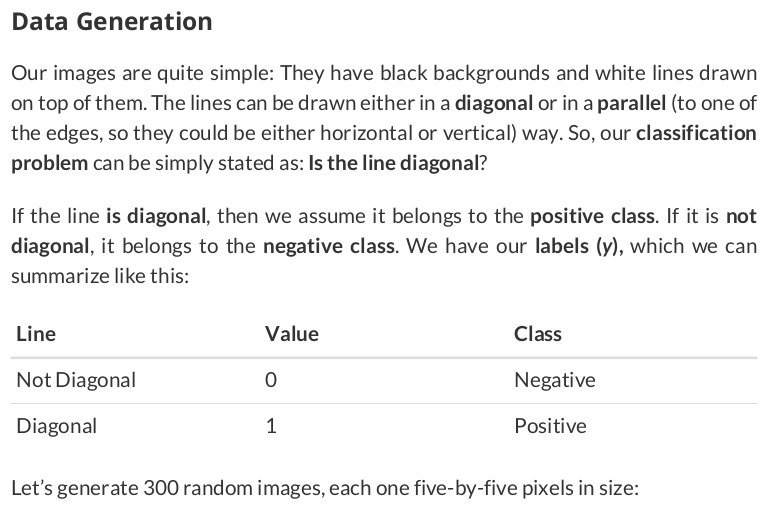
images, labels = generate_dataset(img_size=5, n_images=300, binary=True, seed=13)
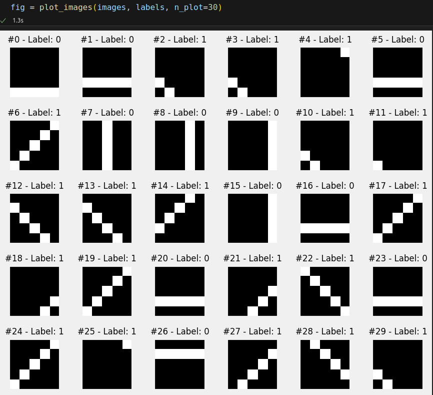
And then let’s visualize the first 30 images:


image_r = np.zeros((5, 5), dtype=np.uint8)
image_r[:, 0] = 255
image_r[:, 1] = 128

image_g = np.zeros((5, 5), dtype=np.uint8)
image_g[:, 1] = 128
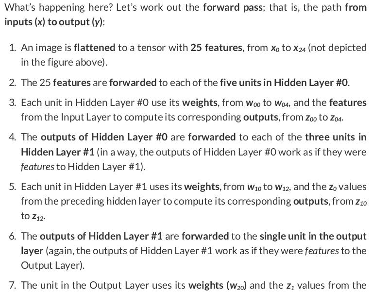
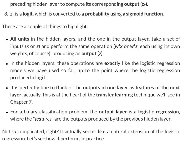
image_g[:, 2] = 255
image_g[:, 3] = 128

image_b = np.zeros((5, 5), dtype=np.uint8)
image_b[:, 3] = 128
image_b[:, 4] = 255
image_r, image_g, image_b
(array([[255, 128,   0,   0,   0],
        [255, 128,   0,   0,   0],
        [255, 128,   0,   0,   0],
        [255, 128,   0,   0,   0],
        [255, 128,   0,   0,   0]], dtype=uint8),
 array([[  0, 128, 255, 128,   0],
        [  0, 128, 255, 128,   0],
        [  0, 128, 255, 128,   0],
        [  0, 128, 255, 128,   0],
        [  0, 128, 255, 128,   0]], dtype=uint8),
 array([[  0,   0,   0, 128, 255],
        [  0,   0,   0, 128, 255],
        [  0,   0,   0, 128, 255],
        [  0,   0,   0, 128, 255],
        [  0,   0,   0, 128, 255]], dtype=uint8))
image_rgb = np.stack([image_r, image_g, image_b], axis=2)
image_rgb
[image_r, image_g, image_b] has shape (3, 5, 5).
array([[[255,   0,   0],
        [128, 128,   0],
        [  0, 255,   0],
        [  0, 128, 128],
        [  0,   0, 255]],

       [[255,   0,   0],
        [128, 128,   0],
        [  0, 255,   0],
        [  0, 128, 128],
        [  0,   0, 255]],

       [[255,   0,   0],
        [128, 128,   0],
        [  0, 255,   0],
        [  0, 128, 128],
        [  0,   0, 255]],

       [[255,   0,   0],
        [128, 128,   0],
        [  0, 255,   0],
        [  0, 128, 128],
        [  0,   0, 255]],

       [[255,   0,   0],
        [128, 128,   0],
        [  0, 255,   0],
        [  0, 128, 128],
        [  0,   0, 255]]], dtype=uint8)
The output has shape (5, 5, 3).
3 5x5 one-channel images were stacked into one 5x5 3-channel image.
fig, ax = plt.subplots(1, 1, figsize=(3, 3))
ax.imshow(image_rgb)
ax.set_xticks([])
ax.set_yticks([])

stacked_on_axis1 = np.stack([image_r, image_g, image_b], axis=1)
stacked_on_axis1
array([[[255, 128,   0,   0,   0],
        [  0, 128, 255, 128,   0],
        [  0,   0,   0, 128, 255]],

       [[255, 128,   0,   0,   0],
        [  0, 128, 255, 128,   0],
        [  0,   0,   0, 128, 255]],

       [[255, 128,   0,   0,   0],
        [  0, 128, 255, 128,   0],
        [  0,   0,   0, 128, 255]],

       [[255, 128,   0,   0,   0],
        [  0, 128, 255, 128,   0],
        [  0,   0,   0, 128, 255]],

       [[255, 128,   0,   0,   0],
        [  0, 128, 255, 128,   0],
        [  0,   0,   0, 128, 255]]], dtype=uint8)
The output has shape (5, 3, 5).
fig, ax = plt.subplots(1, 1, figsize=(3, 3))
ax.imshow(stacked_on_axis1)
ax.set_xticks([])
ax.set_yticks([])
TypeError: Invalid shape (5, 3, 5) for image data
image_gray = (.2126 * image_r + .7152 * image_g + .0722 * image_b).astype(np.uint8)
image_gray
array([[ 54, 118, 182, 100,  18],
       [ 54, 118, 182, 100,  18],
       [ 54, 118, 182, 100,  18],
       [ 54, 118, 182, 100,  18],
       [ 54, 118, 182, 100,  18]], dtype=uint8)
Let’s see what the matrices above represent.



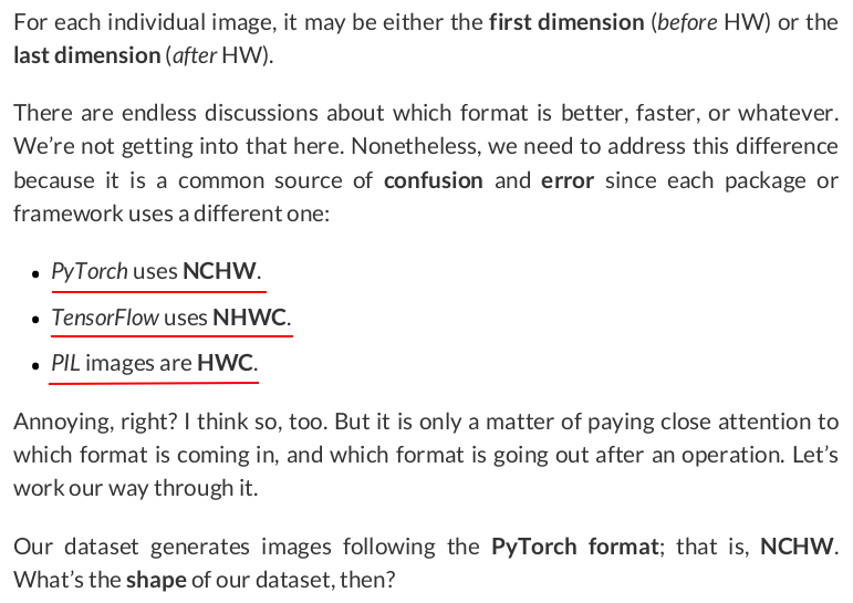
images.shape

# (300, 1, 5, 5)
As expected, 300 images, single-channel, five pixels wide, five pixels high. Let’s take a closer look at one image, say, image #12:
example = images[12]
example
array([[[  0,   0,   0,   0,   0],
        [255,   0,   0,   0,   0],
        [  0, 255,   0,   0,   0],
        [  0,   0, 255,   0,   0],
        [  0,   0,   0, 255,   0]]], dtype=uint8)

example_hwc = np.transpose(example, (1, 2, 0))
example_hwc.shape  # (5, 5, 1)
The shape is correct: HWC. What about the content?


from torchvision.transforms.v2 import ToImage

image_tensor = ToImage()(example_hwc)
image_tensor, image_tensor.shape
(Image([[[  0,   0,   0,   0,   0],
         [255,   0,   0,   0,   0],
         [  0, 255,   0,   0,   0],
         [  0,   0, 255,   0,   0],
         [  0,   0,   0, 255,   0]]], dtype=torch.uint8, ),
 torch.Size([1, 5, 5]))

isinstance(image_tensor, torch.Tensor)

# True
See? It is really a tensor. Now, let’s scale its values:
from torchvision.transforms.v2 import ToDtype

example_tensor = ToDtype(torch.float32, scale=True)(image_tensor)
example_tensor
Image([[[0., 0., 0., 0., 0.],
        [1., 0., 0., 0., 0.],
        [0., 1., 0., 0., 0.],
        [0., 0., 1., 0., 0.],
        [0., 0., 0., 1., 0.]]], )

from torchvision.transforms.v2 import Compose

def ToTensor():
    return Compose([ToImage(), ToDtype(torch.float32, scale=True)])

tensorizer = ToTensor()
example_tensor = tensorizer(example_hwc)
example_tensor
Image([[[0., 0., 0., 0., 0.],
        [1., 0., 0., 0., 0.],
        [0., 1., 0., 0., 0.],
        [0., 0., 1., 0., 0.],
        [0., 0., 0., 1., 0.]]], )
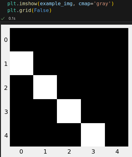
There it is, the same image tensor as before. Moreover, we can "see" the same diagonal line as in the original image. Perhaps you’re wondering what that Compose() method is doing there, but don’t worry, we’ll get to it very soon.


from torchvision.transforms.v2 import ToPILImage

example_img = ToPILImage()(example_tensor)
type(example_img)

# PIL.Image.Image
Notice that it is a real PIL image, not a Numpy array anymore, so we can use Matplotlib to visualize it:

from torchvision.transforms.v2 import RandomHorizontalFlip

flipper = RandomHorizontalFlip(p=1.0)
flipped_img = flipper(example_img)
OK, the image should be flipped horizontally now. Let’s check it out:


img_tensor = tensorizer(flipped_img)
img_tensor
Image([[[0., 0., 0., 0., 0.],
        [0., 0., 0., 0., 1.],
        [0., 0., 0., 1., 0.],
        [0., 0., 1., 0., 0.],
        [0., 1., 0., 0., 0.]]], )


from torchvision.transforms.v2 import Normalize

normalizer = Normalize(mean=(0.5,), std=(0.5,))
normalized_tensor = normalizer(img_tensor)
normalized_tensor
Image([[[-1., -1., -1., -1., -1.],
        [-1., -1., -1., -1.,  1.],
        [-1., -1., -1.,  1., -1.],
        [-1., -1.,  1., -1., -1.],
        [-1.,  1., -1., -1., -1.]]], )

composer = Compose([RandomHorizontalFlip(p=1.0),
                    Normalize(mean=(.5,), std=(.5,))])

composed_tensor = composer(example_tensor)
(composed_tensor == normalized_tensor).all()

# tensor(True)

print(example)
print(example_tensor)
[[[  0   0   0   0   0]
  [255   0   0   0   0]
  [  0 255   0   0   0]
  [  0   0 255   0   0]
  [  0   0   0 255   0]]]
Image([[[0., 0., 0., 0., 0.],
        [1., 0., 0., 0., 0.],
        [0., 1., 0., 0., 0.],
        [0., 0., 1., 0., 0.],
        [0., 0., 0., 1., 0.]]], )

example_tensor = torch.as_tensor(example / 255).float()


# Build tensors from numpy arrays BEFORE split
x_tensor = torch.as_tensor(images / 255).float()
y_tensor = torch.as_tensor(labels.reshape(-1, 1)).float()


class TransformedTensorDataset(Dataset):
    def __init__(self, x, y, transform=None):
        self.x = x
        self.y = y
        self.transform = transform

    def __getitem__(self, index):
        x = self.x[index]

        if self.transform:
            x = self.transform(x)

        return x, self.y[index]

    def __len__(self):
        return len(self.x)
composer = Compose([RandomHorizontalFlip(p=.5),
                    Normalize(mean=(.5,), std=(.5,))])

dataset = TransformedTensorDataset(x_tensor, y_tensor, transform=composer)
Cool! But we still have to split the dataset as usual. But we’ll do it a bit differently this time.
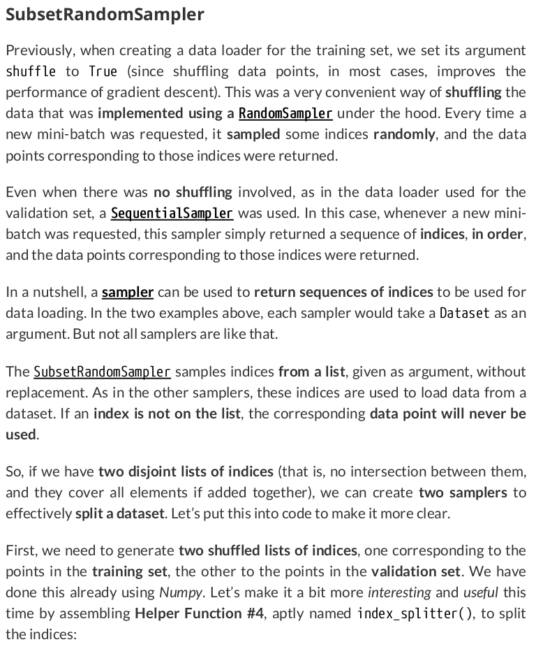
from torch.utils.data import random_split


def index_splitter(n, splits, seed=13):
    '''
    Parameters:
    n: The number of data points to generate indices for.
    splits: A list of values representing the relative weights of the split sizes.
    seed: A random seed to ensure reproducibility.
    '''

    idx = torch.arange(n)

    # Make the splits argument a tensor
    splits_tensor = torch.as_tensor(splits)
    total = splits_tensor.sum().float()

    # If the total does not add up to one, divide every number by the total.
    if not total.isclose(torch.tensor(1.)):
        splits_tensor = splits_tensor / total

    # Use PyTorch random_split to split the indices
    torch.manual_seed(seed)
    return random_split(idx, splits_tensor)
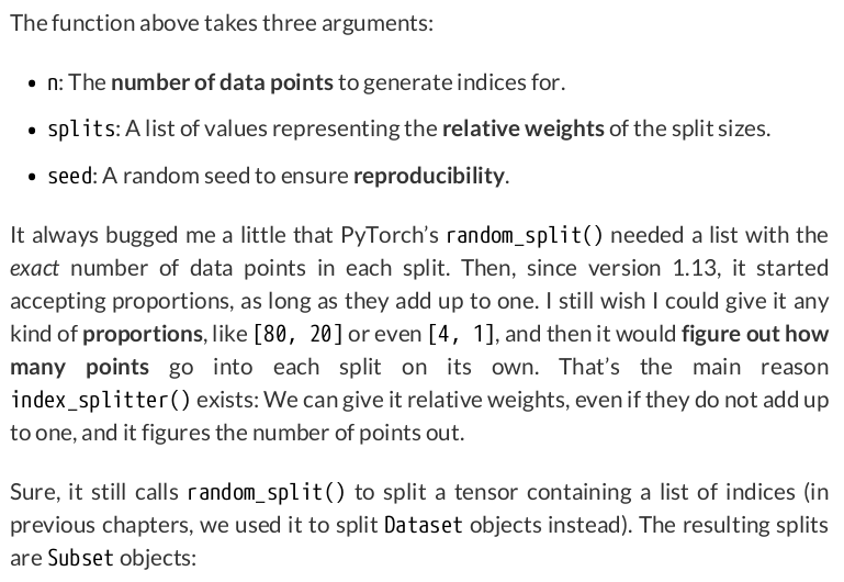
train_idx, val_idx = index_splitter(len(x_tensor), [80, 20])
train_idx

# <torch.utils.data.dataset.Subset at 0x7586de8747d0>
Each subset contains the corresponding indices as an attribute:

Next, each Subset object is used as an argument to the corresponding sampler:
from torch.utils.data import SubsetRandomSampler


train_sampler = SubsetRandomSampler(train_idx)
val_sampler = SubsetRandomSampler(val_idx)

train_loader = DataLoader(dataset=dataset, batch_size=16, sampler=train_sampler)
val_loader = DataLoader(dataset=dataset, batch_size=16, sampler=val_sampler)

We can also check if the loaders are returning the correct number of mini-batches:
len(iter(train_loader)), len(iter(val_loader))

# (15, 4)


# Uses indices to perform the split
x_train_tensor = x_tensor[train_idx]
y_train_tensor = y_tensor[train_idx]

x_val_tensor = x_tensor[val_idx]
y_val_tensor = y_tensor[val_idx]

train_composer = Compose([RandomHorizontalFlip(p=0.5),
                          Normalize(mean=(0.5,), std=(0.5,))])
val_composer = Compose([Normalize(mean=(0.5,), std=(0.5,))])
Next, we use them to create two datasets and their corresponding data loaders:
train_dataset = TransformedTensorDataset(x_train_tensor, y_train_tensor, transform=train_composer)
val_dataset = TransformedTensorDataset(x_val_tensor, y_val_tensor, transform=val_composer)

train_loader = DataLoader(dataset=train_dataset, batch_size=16, shuffle=True)
val_loader = DataLoader(dataset=val_dataset, batch_size=16)

classes, counts = y_train_tensor.unique(return_counts=True)
print(classes, counts)

# tensor([0., 1.]) tensor([ 72, 168])
Ours is a binary classification, so it is no surprise we have two classes: zero (not diagonal) and one (diagonal). There are 72 images with lines that are not diagonal, and 168 images with diagonal lines. Clearly, an imbalanced dataset.
Next, we compute the weights by inverting the counts. It is as simple as that:
weights = 1. / counts.float()
weights

# tensor([0.0139, 0.0060])
The first weight (0.0139) corresponds to the negative class (not diagonal). Since this class has only 72 out of 240 images in our training set, it is also the minority class. The other weight (0.0060) corresponds to the positive class (diagonal), which has the remaining 168 images, thus making it the majority class.
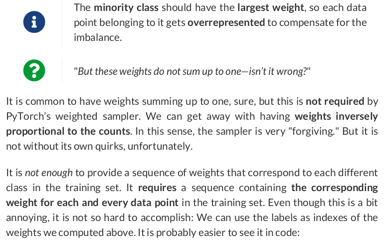
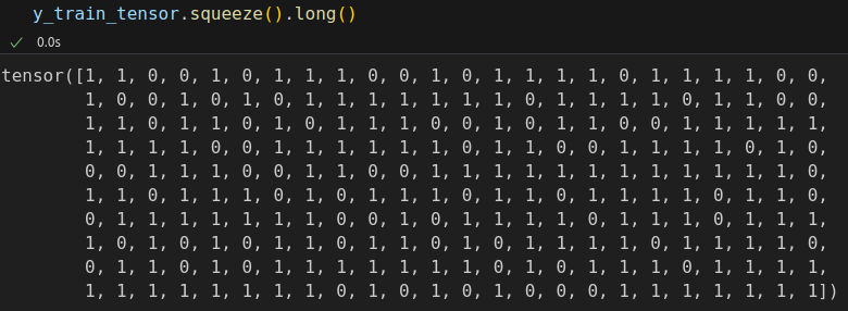

Since there are 240 images in our training set, we need 240 weights. We squeeze our labels (y_train_tensor) to a single dimension and cast them to long type since we want to use them as indices.

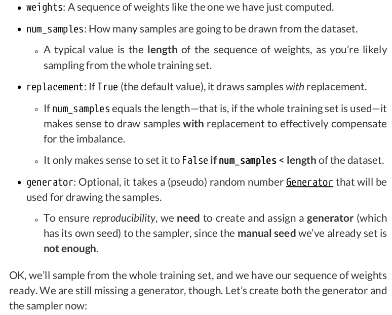
from torch.utils.data import WeightedRandomSampler


generator = torch.Generator()

sampler = WeightedRandomSampler(
    weights=sample_weights,
    num_samples=len(sample_weights),
    generator=generator,
    replacement=True
)

train_loader = DataLoader(dataset=train_dataset, batch_size=16, sampler=sampler)
val_loader = DataLoader(dataset=val_dataset, batch_size=16)

def make_balanced_sampler(y):
    # Compute weights for compensating imbalanced classes
    classes, counts = y.unique(return_counts=True)
    weights = 1. / counts.float()
    sample_weights = weights[y.squeeze().long()]

    generator = torch.Generator()

    # Build the weighted sampler
    sampler = WeightedRandomSampler(
        weights=sample_weights,
        num_samples=len(sample_weights),
        generator=generator,
        replacement=True
    )

    return sampler
sampler = make_balanced_sampler(y_train_tensor)

train_loader.sampler.generator.manual_seed(42)

torch.tensor([t[1].sum() for t in iter(train_loader)]).sum()

# tensor(121.)
Close enough! We have 168 images of the positive class, and now, thanks to the weighted sampler, we’re sampling only 121 of them. It means we’re oversampling the negative class (which has 72 images) to a total of 119 images, adding up to 240
images. Mission accomplished, our dataset is balanced now.
Update the set_seed() method in class StepByStep:
    def set_seed(self, seed=42):
        torch.backends.cudnn.deterministic = True
        torch.backends.cudnn.benchmark = False
        torch.manual_seed(seed)
        try:
            self.train_loader.sampler.generator.manual_seed(seed)
        except AttributeError:
            pass
Our updated method tries to update the seed of the generator used by the sampler assigned to the data loader of the training set. But, if there is no generator (the argument is optional, after all), it fails silently.
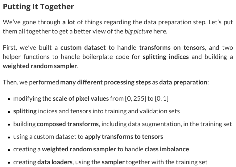
# Build tensors from numpy arrays BEFORE split
# Modify the scale of pixel values from [0, 255] to [0, 1]
x_tensor = torch.as_tensor(images / 255).float()
y_tensor = torch.as_tensor(labels.reshape(-1, 1)).float()

# Use index_splitter to generate indices for training and validation sets
train_idx, val_idx = index_splitter(len(x_tensor), [80, 20])

# Use indices to perform the split
x_train_tensor = x_tensor[train_idx]
y_train_tensor = y_tensor[train_idx]
x_val_tensor = x_tensor[val_idx]
y_val_tensor = y_tensor[val_idx]

# Build different composers because of data augmentation on training set
train_composer = Compose([RandomHorizontalFlip(p=.5),
                          Normalize(mean=(.5,), std=(.5,))])
val_composer = Compose([Normalize(mean=(.5,), std=(.5,))])

# Use custom dataset to apply composed transforms to each set
train_dataset = TransformedTensorDataset(x_train_tensor, y_train_tensor, transform=train_composer)
val_dataset = TransformedTensorDataset(x_val_tensor, y_val_tensor, transform=val_composer)

# Build a weighted random sampler to handle imbalanced classes
sampler = make_balanced_sampler(y_train_tensor)

# Use sampler in the training set to get a balanced data loader
train_loader = DataLoader(dataset=train_dataset, batch_size=16, sampler=sampler)
val_loader = DataLoader(dataset=val_dataset, batch_size=16)

Let’s take one mini-batch of images from our training set to illustrate how it works:
dummy_xs, dummy_ys = next(iter(train_loader))
dummy_xs.shape

# torch.Size([16, 1, 5, 5])
Our dummy mini-batch has 16 images, one channel each, dimensions five-by-five pixels. What if we flatten this mini-batch?
flattener = nn.Flatten()
dummy_xs_flat = flattener(dummy_xs)

print(dummy_xs_flat.shape)
print(dummy_xs_flat[0])
torch.Size([16, 25])
tensor([-1.,  1., -1., -1., -1., -1.,  1., -1., -1., -1., -1.,  1., -1., -1.,
        -1., -1.,  1., -1., -1., -1., -1.,  1., -1., -1., -1.])


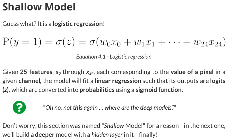
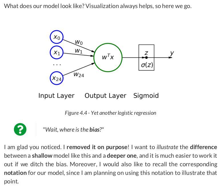

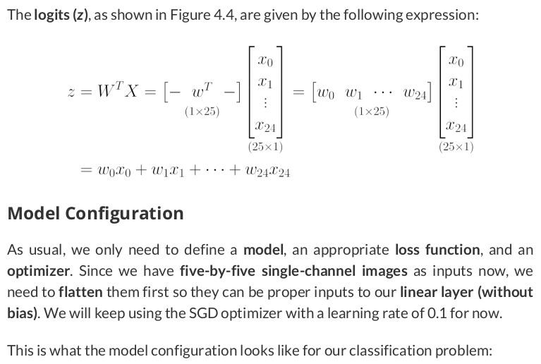
# Learning rate
lr = .1

torch.manual_seed(17)

# Create a model
model_logistic = nn.Sequential()
model_logistic.add_module('flatten', nn.Flatten())
model_logistic.add_module('output', nn.Linear(25, 1, bias=False))
model_logistic.add_module('sigmoid', nn.Sigmoid())

# Define a SGD optimizer to update the parameters
optimizer_logistic = optim.SGD(model_logistic.parameters(), lr=lr)

# Define a binary cross entropy loss function
bce_loss_fn = nn.BCELoss()

n_epochs = 100

sbs_logistic = StepByStep(model_logistic, bce_loss_fn, optimizer_logistic)
sbs_logistic.set_loaders(train_loader, val_loader)
sbs_logistic.train(n_epochs)
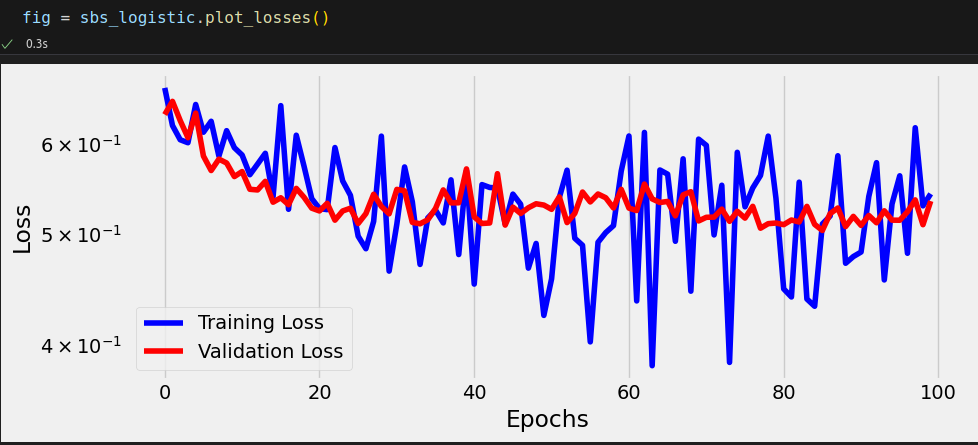
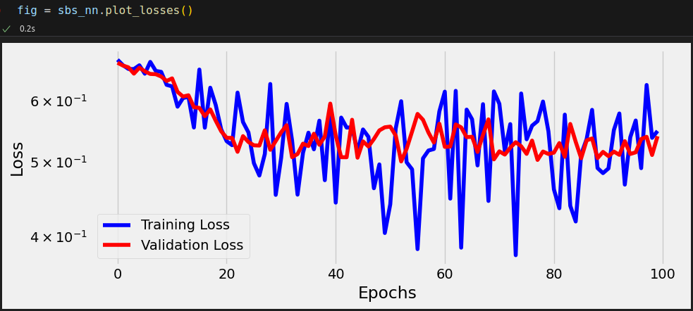
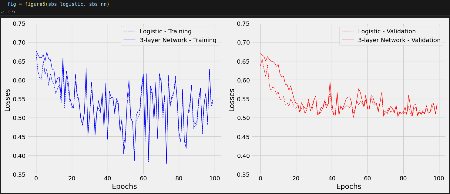
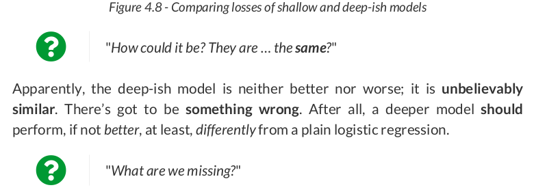
Awful, right? It seems our model is barely learning anything! Maybe a deeper model can do better.

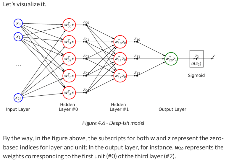

# Learning rate
lr = .1

torch.manual_seed(17)

# Creae a model
model_nn = nn.Sequential()
model_nn.add_module('flatten', nn.Flatten())
model_nn.add_module('hidden0', nn.Linear(25, 5, bias=False))
model_nn.add_module('hidden1', nn.Linear(5, 3, bias=False))
model_nn.add_module('output', nn.Linear(3, 1, bias=False))
model_nn.add_module('sigmoid', nn.Sigmoid())

# Define a SGD optimizer to update the parameters
optimizer_nn = optim.SGD(model_nn.parameters(), lr=lr)

# Define a binary cross entropy loss function
bce_loss_fn = nn.BCELoss()







w_nn_hidden0 = model_nn.hidden0.weight.detach()
w_nn_hidden1 = model_nn.hidden1.weight.detach()
w_nn_output = model_nn.output.weight.detach()

w_nn_hidden0.shape, w_nn_hidden1.shape, w_nn_output.shape

# (torch.Size([5, 25]), torch.Size([3, 5]), torch.Size([1, 3]))

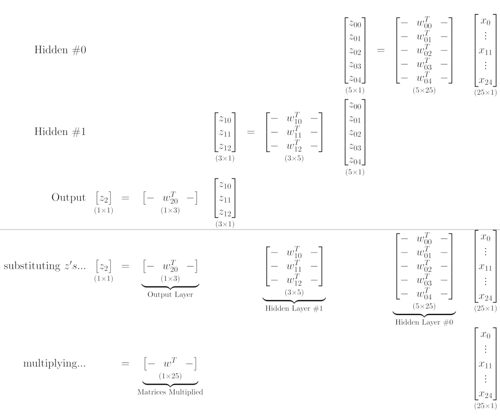
w_nn_equiv = w_nn_output @ w_nn_hidden1 @ w_nn_hidden0
w_nn_equiv.shape

# torch.Size([1, 25])

w_nn_equiv = w_nn_output.mm(w_nn_hidden1.mm(w_nn_hidden0))

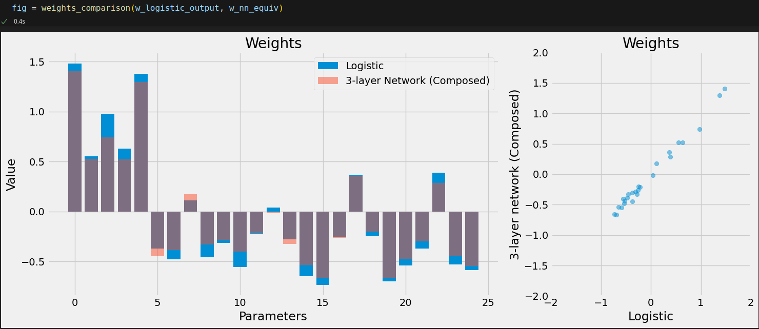
w_logistic_output = model_logistic.output.weight.detach()
w_logistic_output.shape

# torch.Size([1, 25])


def count_parameters(self):
    return sum(p.numel() for p in self.model.parameters() if p.requires_grad)

setattr(StepByStep, 'count_parameters', count_parameters)

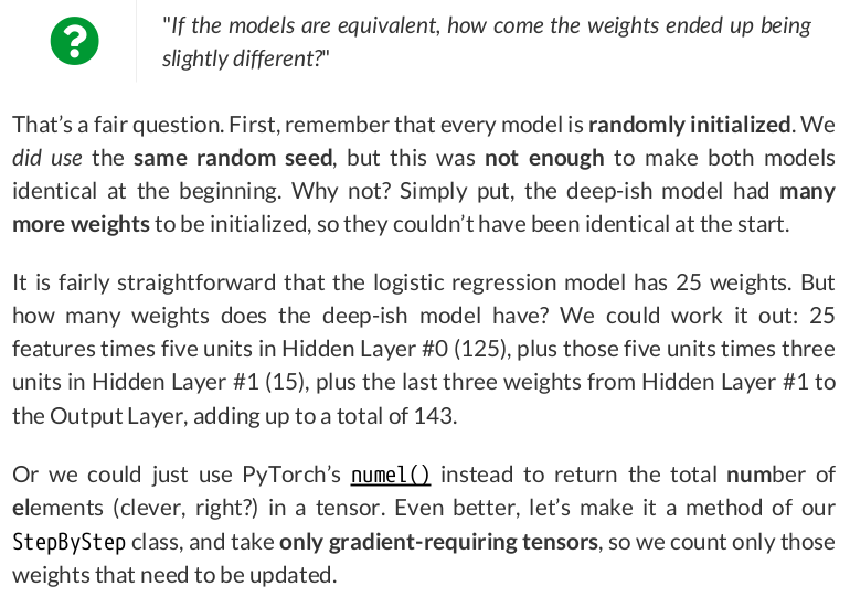
sbs_logistic.count_parameters(), sbs_nn.count_parameters()

# (25, 143)

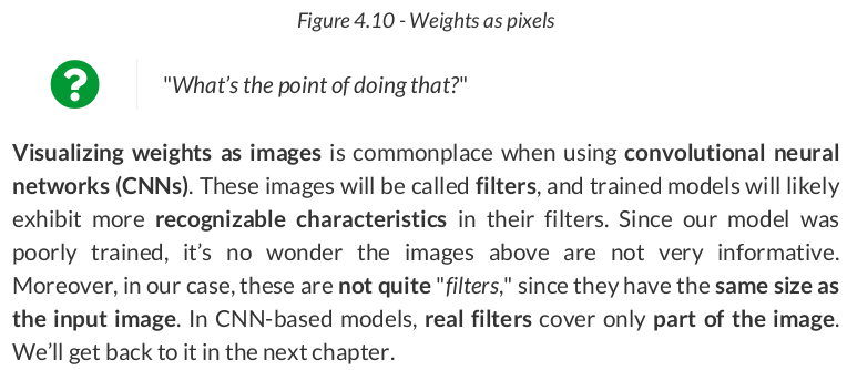
w_nn_hidden0.shape

# torch.Size([5, 25])





dummy_z = torch.tensor([-3., 0., 3.])

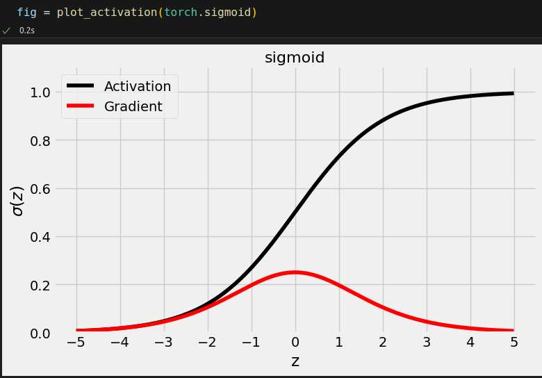
torch.sigmoid(dummy_z)  # tensor([0.0474, 0.5000, 0.9526])

nn.Sigmoid()(dummy_z)  # tensor([0.0474, 0.5000, 0.9526])

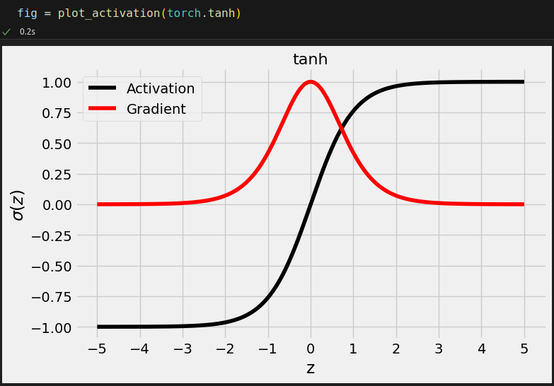

dummy_z = torch.tensor([-3., 0., 3.])

torch.tanh(dummy_z)  # tensor([-0.9951,  0.0000,  0.9951])

nn.Tanh()(dummy_z)  # tensor([-0.9951,  0.0000,  0.9951])
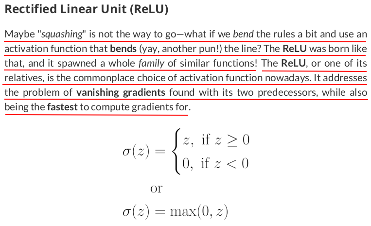
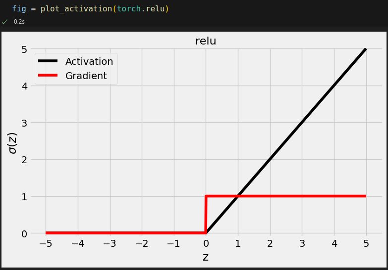

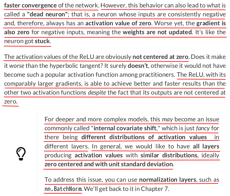
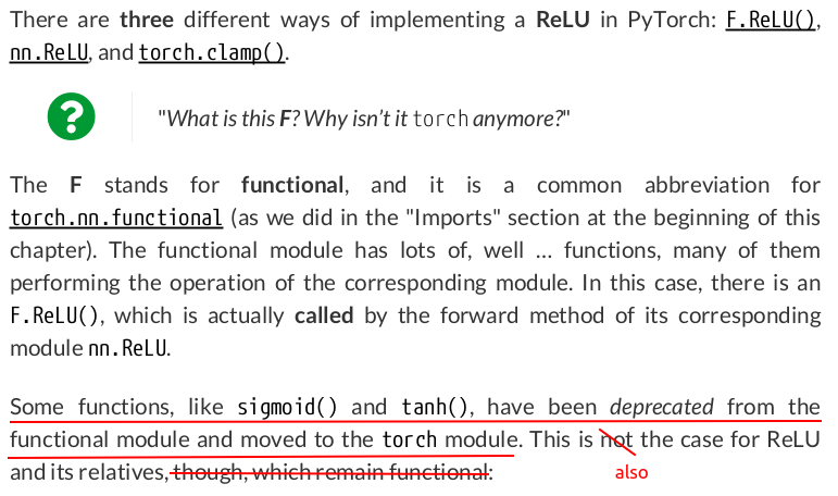
import torch.nn.functional as F


dummy_z = torch.tensor([-3., 0., 3.])
torch.relu(dummy_z)  # tensor([0., 0., 3.])

F.relu(dummy_z)  # tensor([0., 0., 3.])

nn.ReLU()(dummy_z)  # tensor([0., 0., 3.])

dummy_z.clamp(min=0)  # tensor([0., 0., 3.])
And, in the particular case of the ReLU, we can use clamp() to directly cap z at a minimum value of zero.
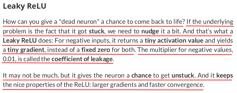

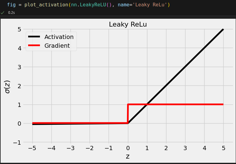

(There's no torch.leaky_relu() yet.)
dummy_z = torch.tensor([-3., 0., 3.])

F.leaky_relu(dummy_z, negative_slope=.01)  # tensor([-0.0300,  0.0000,  3.0000])

nn.LeakyReLU(negative_slope=.02)(dummy_z)  # tensor([-0.0600,  0.0000,  3.0000])

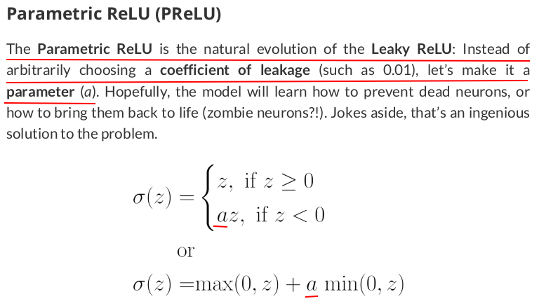
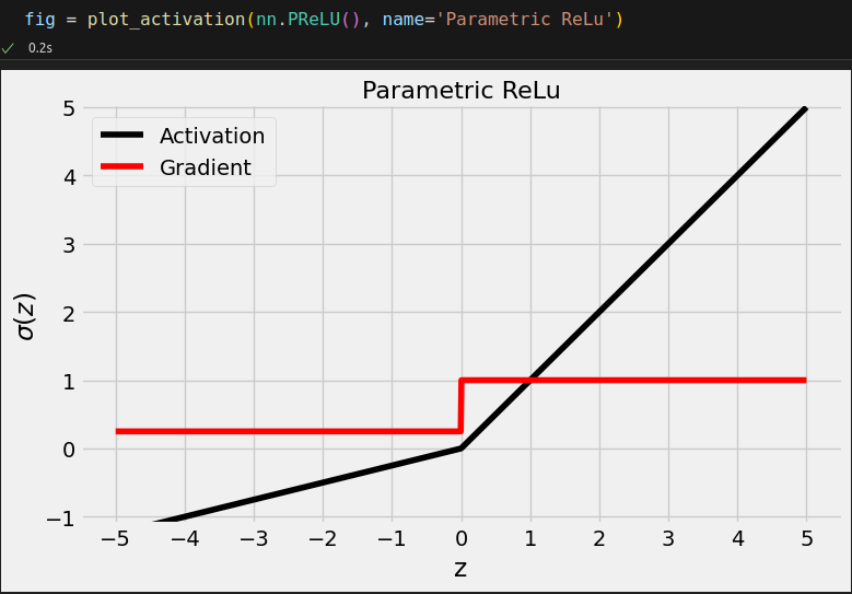


dummy_z = torch.tensor([-3., 0., 3.])

F.prelu(dummy_z, weight=torch.tensor(0.25))  # tensor([-0.7500,  0.0000,  3.0000])

nn.PReLU(init=0.25)(dummy_z) # tensor([-0.7500, 0.0000, 3.0000], grad_fn=<PreluKernelBackward0>)
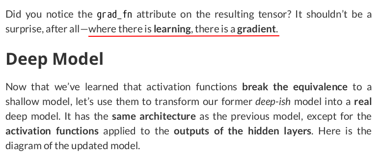
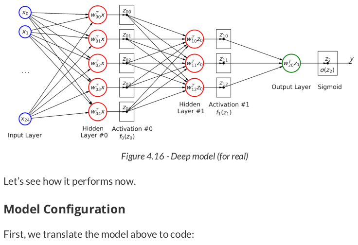
lr = .1

torch.manual_seed(17)

model_relu = nn.Sequential()
model_relu.add_module('flatten', nn.Flatten())
model_relu.add_module('hidden0', nn.Linear(25, 5, bias=False))
model_relu.add_module('activation0', nn.ReLU())
model_relu.add_module('hidden1', nn.Linear(5, 3, bias=False))
model_relu.add_module('activation1', nn.ReLU())
model_relu.add_module('output', nn.Linear(3, 1, bias=False))
model_relu.add_module('sigmoid', nn.Sigmoid())

optimizer_relu = optim.SGD(model_relu.parameters(), lr=lr)

bce_loss_fn = nn.BCELoss()
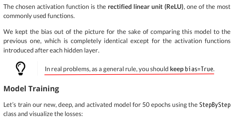
n_epochs = 50

sbs_relu = StepByStep(model_relu, bce_loss_fn, optimizer_relu)
sbs_relu.set_loaders(train_loader, val_loader)
sbs_relu.train(n_epochs)

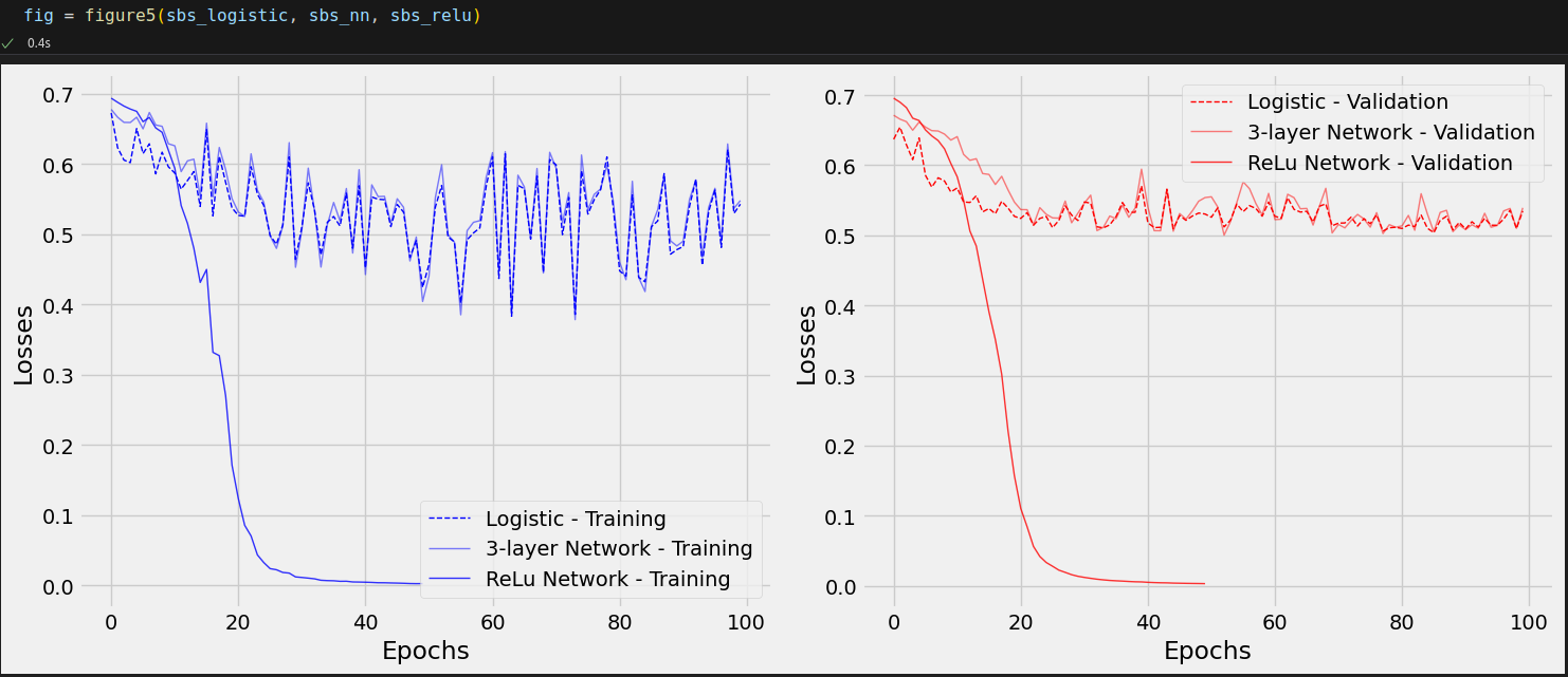
This is more like it! But, to really grasp the difference made by the activation functions, let’s plot all models on the same chart.

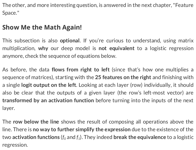
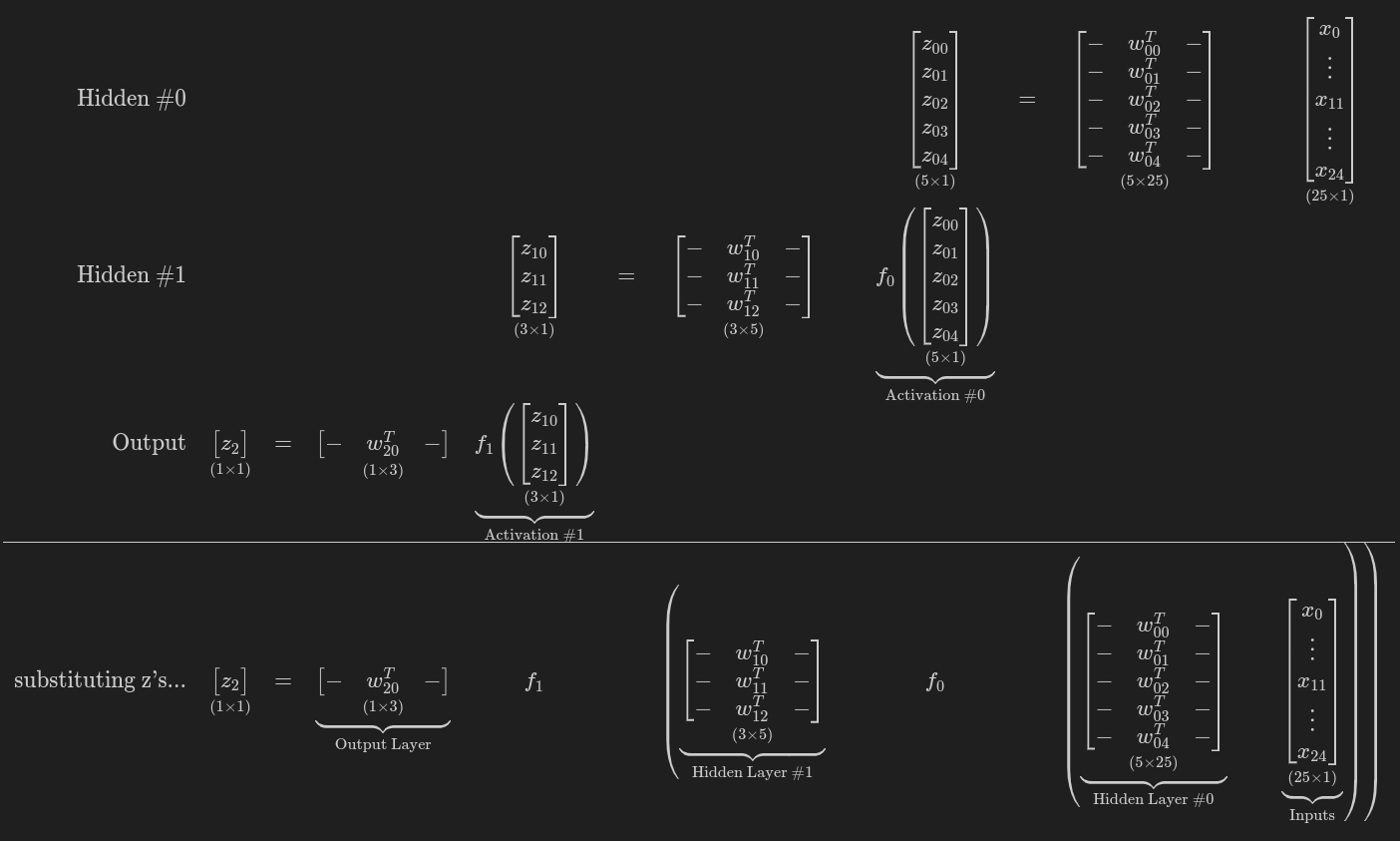
Equation 4.3 - Activation functions break the equivalence
class TransformedTensorDataset(Dataset):
    def __init__(self, x, y, transform=None):
        self.x = x
        self.y = y
        self.transform = transform

    def __getitem__(self, index):
        x = self.x[index]

        if self.transform:
            x = self.transform(x)

        return x, self.y[index]

    def __len__(self):
        return len(self.x)
def index_splitter(n, splits, seed=13):
    '''
    Parameters:
    n: The number of data points to generate indices for.
    splits: A list of values representing the relative weights of the split sizes.
    seed: A random seed to ensure reproducibility.
    '''

    idx = torch.arange(n)

    # Make the splits argument a tensor
    splits_tensor = torch.as_tensor(splits)
    total = splits_tensor.sum().float()

    # If the total does not add up to one, divide every number by the total.
    if not total.isclose(torch.tensor(1.)):
        splits_tensor = splits_tensor / total

    # Use PyTorch random_split to split the indices
    torch.manual_seed(seed)
    return random_split(idx, splits_tensor)
def make_balanced_sampler(y):
    # Compute weights for compensating imbalanced classes
    classes, counts = y.unique(return_counts=True)
    weights = 1. / counts.float()
    sample_weights = weights[y.squeeze().long()]

    generator = torch.Generator()

    # Build the weighted sampler
    sampler = WeightedRandomSampler(
        weights=sample_weights,
        num_samples=len(sample_weights),
        generator=generator,
        replacement=True
    )

    return sampler
# Build tensors from numpy arrays BEFORE split
# Modify the scale of pixel values from [0, 255] to [0, 1]
x_tensor = torch.as_tensor(images / 255).float()
y_tensor = torch.as_tensor(labels.reshape(-1, 1)).float()

# Use index_splitter to generate indices for training and validation sets
train_idx, val_idx = index_splitter(len(x_tensor), [80, 20])

# Use indices to perform the split
x_train_tensor = x_tensor[train_idx]
y_train_tensor = y_tensor[train_idx]
x_val_tensor = x_tensor[val_idx]
y_val_tensor = y_tensor[val_idx]

# Build different composers because of data augmentation on training set
train_composer = Compose([RandomHorizontalFlip(p=.5),
                          Normalize(mean=(.5,), std=(.5,))])
val_composer = Compose([Normalize(mean=(.5,), std=(.5,))])

# Use custom dataset to apply composed transforms to each set
train_dataset = TransformedTensorDataset(x_train_tensor, y_train_tensor, transform=train_composer)
val_dataset = TransformedTensorDataset(x_val_tensor, y_val_tensor, transform=val_composer)

# Build a weighted random sampler to handle imbalanced classes
sampler = make_balanced_sampler(y_train_tensor)

# Use sampler in the training set to get a balanced data loader
train_loader = DataLoader(dataset=train_dataset, batch_size=16, sampler=sampler)
val_loader = DataLoader(dataset=val_dataset, batch_size=16)
lr = .1

torch.manual_seed(17)

model_relu = nn.Sequential()
model_relu.add_module('flatten', nn.Flatten())
model_relu.add_module('hidden0', nn.Linear(25, 5, bias=False))
model_relu.add_module('activation0', nn.ReLU())
model_relu.add_module('hidden1', nn.Linear(5, 3, bias=False))
model_relu.add_module('activation1', nn.ReLU())
model_relu.add_module('output', nn.Linear(3, 1, bias=False))
model_relu.add_module('sigmoid', nn.Sigmoid())

optimizer_relu = optim.SGD(model_relu.parameters(), lr=lr)

bce_loss_fn = nn.BCELoss()
n_epochs = 50

sbs_relu = StepByStep(model_relu, bce_loss_fn, optimizer_relu)
sbs_relu.set_loaders(train_loader, val_loader)
sbs_relu.train(n_epochs)


