Gradient descent is an iterative technique commonly used in machine learning and deep learning to find the best possible set of parameters / coefficients for a given model, data points, and loss function, starting from an initial, and usually random, guess.
In deep learning, we are usually trying to minimize a loss function (also called a cost function), which measures how wrong the model's predictions are.
-
Gradient Descent moves downhill on the loss surface — toward smaller loss values — by stepping in the negative direction of the gradient.
-
Gradient Ascent would move uphill, which would maximize the function — not what we want, because a bigger loss is worse!
In short:
-
We use gradient descent because we want to minimize the loss, not maximize it.
-
If we were solving a problem where we wanted to maximize something (like maximizing reward in reinforcement learning), then gradient ascent could be used instead.
Quick analogy:
Imagine standing on a mountain (the loss function).
-
If you want to reach the valley (minimum loss), you walk down (descent).
-
If you want to climb to the peak (maximum value), you walk up (ascent).


import numpy as np


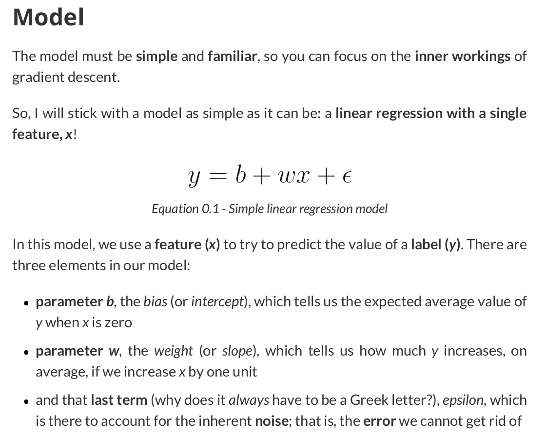
true_b = 1
true_w = 2
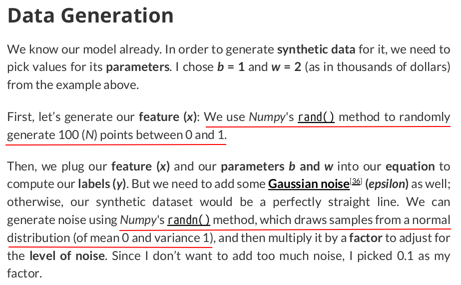
N = 100

# Data Generationrng = np.random.default_rng(54321)
x = rng.random(N)
epsilon = (0.1 * rng.standard_normal(N))
y = true_b + true_w * x + epsilon
print(x.shape)
print(y.shape)
(100,)
(100,)

# Shuffle the indices
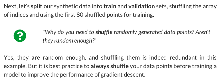
idx = np.arange(N)
np.random.shuffle(idx)

# Use first 80 random indices for train
train_idx = idx[:int(N * 0.8)]
# Use the ramaining indices for validation
val_idx = idx[int(N * 0.8):]

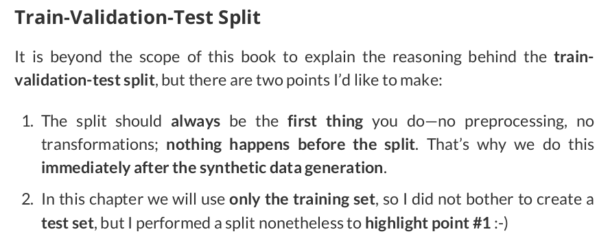
# Generate train and validation sets
x_train, y_train = x[train_idx], y[train_idx]
x_val, y_val = x[val_idx], y[val_idx]


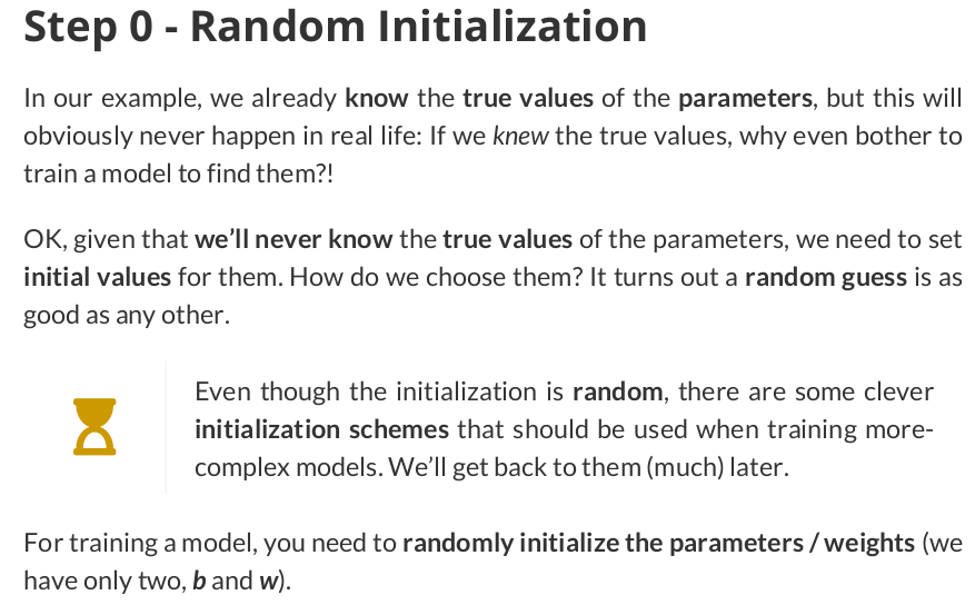
# Step 0 - Initialize parameters "b" and "w" randomly
rng = np.random.default_rng(54321)
b = rng.standard_normal(1)
w = rng.standard_normal(1)

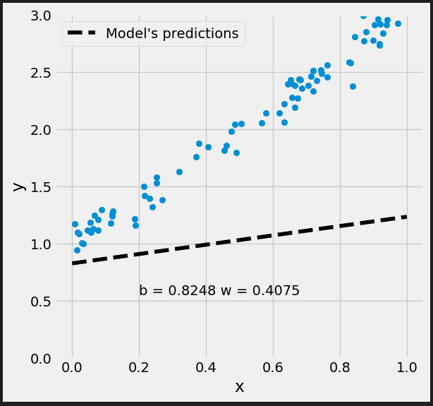
print(b, w) # [0.82483768] [0.40749068]

# Step 1 - Compute our model's predicted output - forward pass
yhat = b + w * x_train
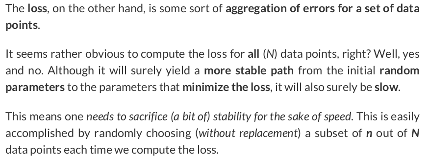
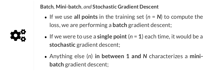
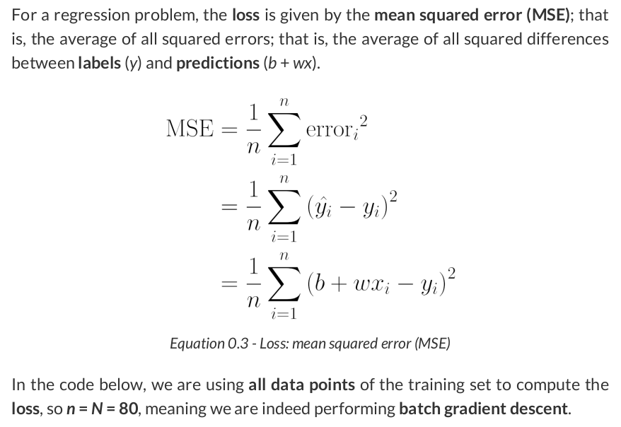
# Step 2 - Compute the loss
# We are using ALL data points, so this is BATCH gradient descent.
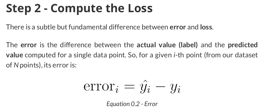
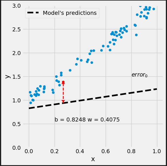
# How wrong is our model? That's the error!
error = yhat - y_train

# It is a regression, so it computes mean squared error (MSE)
loss = (error ** 2).mean()

# Reminder:
# true_b = 1
# true_w = 2

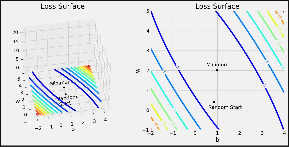
# We have to split the ranges in 100 evenly spaced intervals each.
# Sure, we’re somewhat cheating here, since we know the true values of b and w, so we can
# choose the perfect ranges for the parameters. But it is for educational purposes only.
b_range = np.linspace(true_b - 3, true_b + 3, 101)
w_range = np.linspace(true_w - 3, true_w + 3, 101)
# meshgrid is a handy function that generates a grid of b and w values for all combinations
bs, ws = np.meshgrid(b_range, w_range)
bs.shape, ws.shape  # ((101, 101), (101, 101))
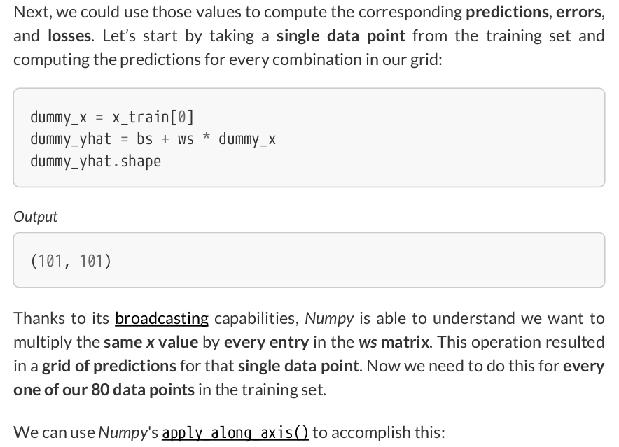
print(x_train.reshape(-1, 1).shape)

# (80, 1)
all_predictions = np.apply_along_axis(
    func1d=lambda x: bs + ws * x,
    axis=1,
    arr=x_train.reshape(-1, 1),
)
all_predictions.shape # (80, 101, 101)

all_labels = y_train.reshape(-1, 1, 1)
all_labels.shape # (80, 1, 1)

all_errors = all_predictions - all_labels
all_errors.shape # (80, 101, 101)
Each prediction has its own error, so we get 80 matrices of shape (101, 101), again, one matrix for each data point, each matrix containing a grid of errors.

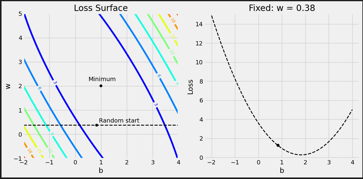
all_losses = (all_errors ** 2).mean(axis=0)
all_losses.shape # (101, 101)





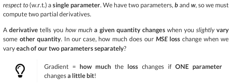
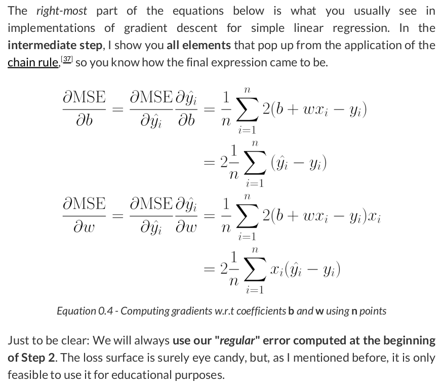
# Step 3 - Compute gradients for both "b" and "w" parameters
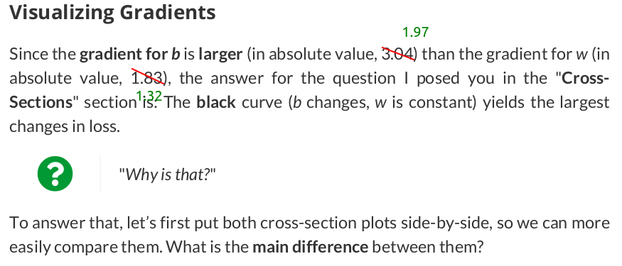
b_grad = 2 * error.mean()
w_grad = 2 * (x_train * error).mean()
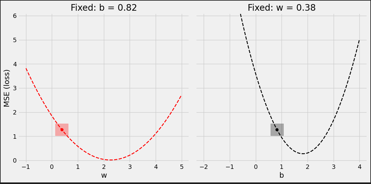
print(b_grad, w_grad) # -1.965279236007916 -1.3213968667849743


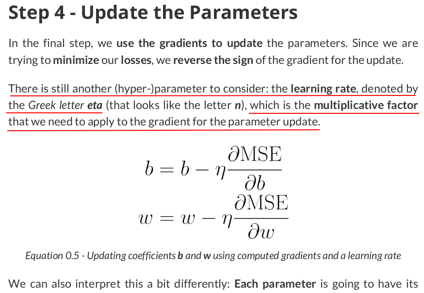

以gradients作为learning rate的权重来更新parameters.

# Set learning rate - this is "eta"
lr = .1
print(b, w)
# [0.82483768] [0.40749068]

# Step 4 - Update parameters using gradients and the learning rate
b = b - lr * b_grad
w = w - lr * w_grad

print(b, w)
# [1.02136561] [0.53963036]

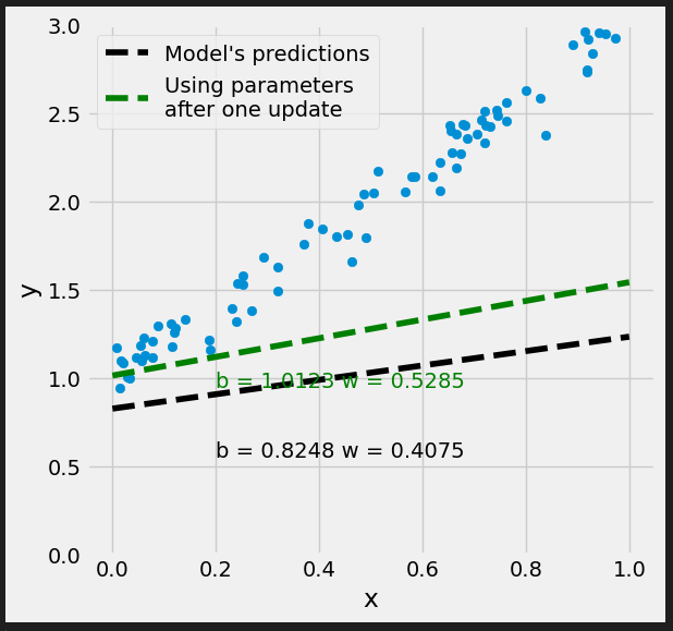
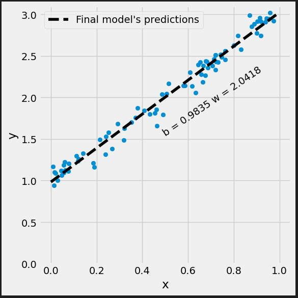
Figure 0.9 - Updated model’s predictions
It looks better.





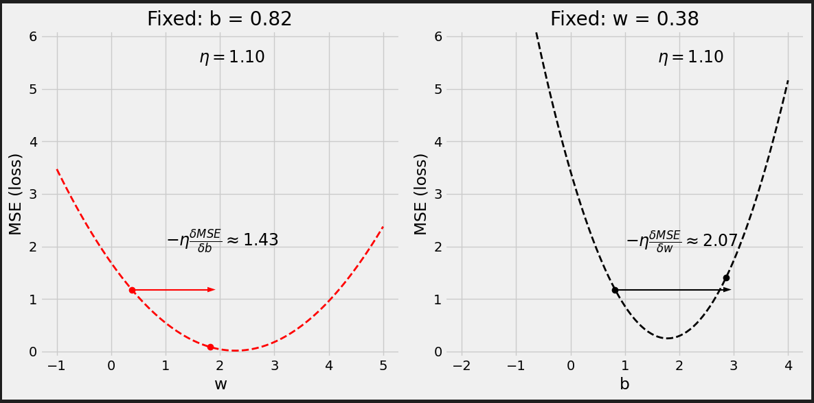
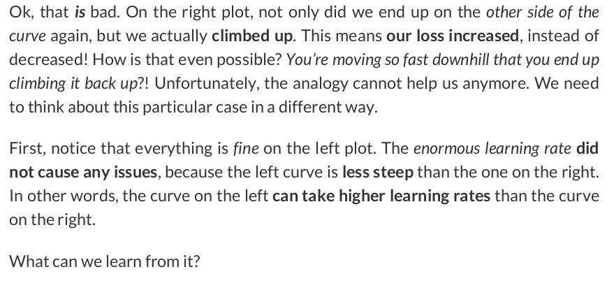
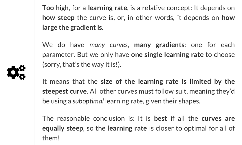
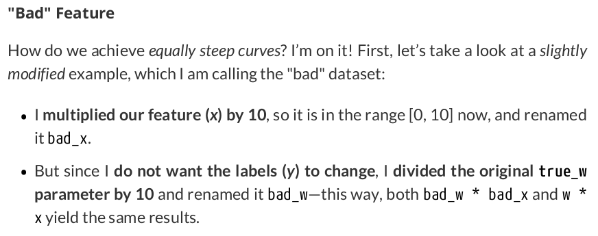
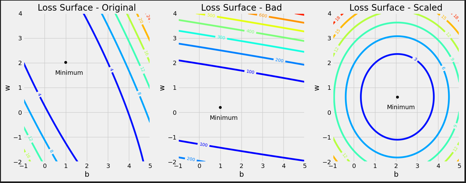
true_b = 1
true_w = 2
N = 100

# Data Generation
rng = np.random.default_rng(54321)

# We divide w by 10
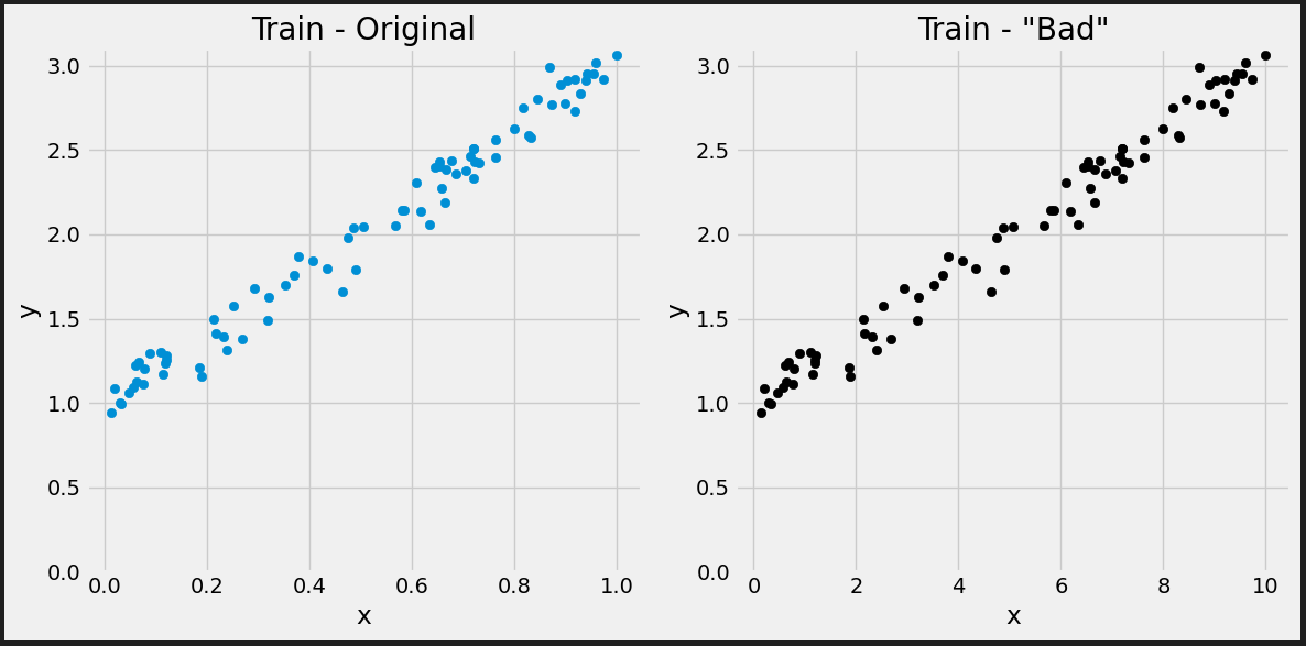
bad_w = true_w / 10
# And multiply x by 10
bad_x = rng.random(N) * 10

epsilon = 0.1 * rng.standard_normal(N)

# So, the net effect on y is zero - it is still the same as before
y = true_b + bad_w * bad_x + epsilon

# Generate train and validation sets
# Use the same train_idx and val_idx as before, but apply to bad_x
bad_x_train, y_train = bad_x[train_idx], y[train_idx]
bad_x_val, y_val = bad_x[val_idx], y[val_idx]





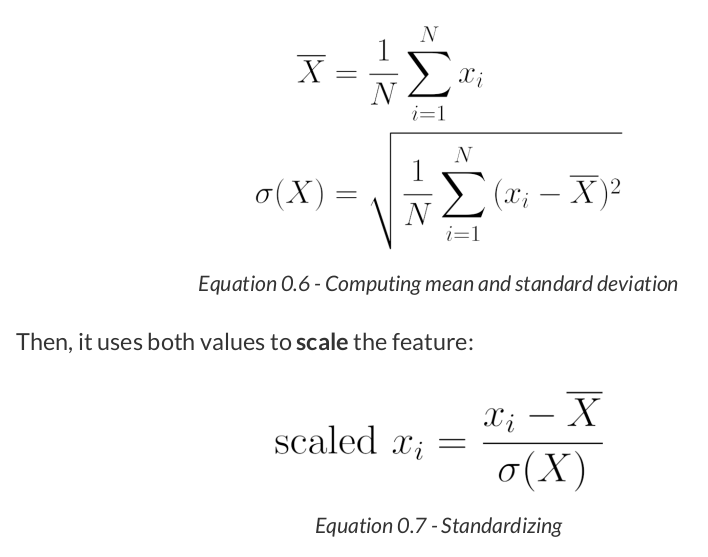
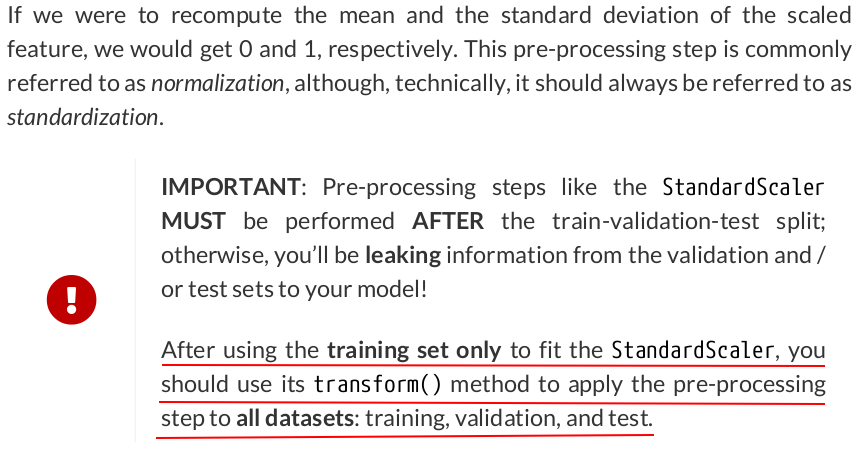
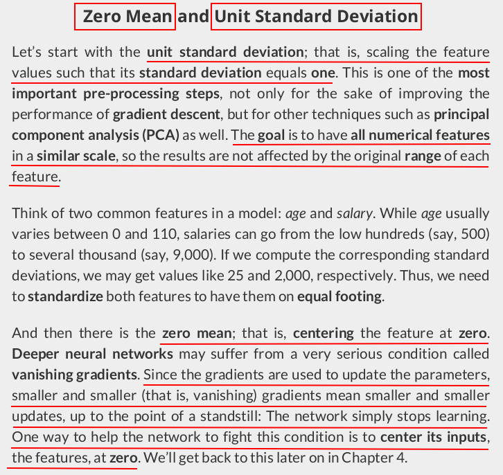
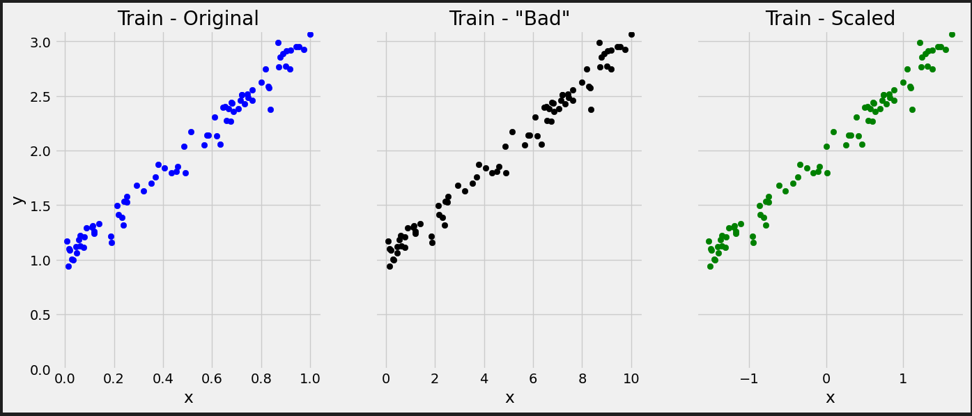
from sklearn.preprocessing import StandardScaler


scaler = StandardScaler(with_mean=True, with_std=True)
# We use the TRAIN set ONLY to fit the scaler
scaler.fit(x_train.reshape(-1, 1))

# Now we can use the already fit scaler to TRANSFORM both TRAIN and VALIDATION sets
scaled_x_train = scaler.transform(x_train.reshape(-1, 1))
scaled_x_val = scaler.transform(x_val.reshape(-1, 1))











 浙公网安备 33010602011771号