1、pytorch_geometric基本使用

1、工具包安装方法：

• 一定参考其GITHUB：https://github.com/pyg-team/pytorch_geometric
  (千万不要pip直接安装，肯定不行的)
  （1）先安装编译好的包：
  https://data.pyg.org/whl/
  （2）再安装整体
  pip install torch_geometric

%matplotlib inline
import torch
import networkx as nx
import matplotlib.pyplot as plt


def visualize_graph(G, color):
    plt.figure(figsize=(7,7))
    plt.xticks([])
    plt.yticks([])
    nx.draw_networkx(G, pos=nx.spring_layout(G, seed=42), with_labels=False,
                     node_color=color, cmap="Set2")
    plt.show()


def visualize_embedding(h, color, epoch=None, loss=None):
    plt.figure(figsize=(7,7))
    plt.xticks([])
    plt.yticks([])
    h = h.detach().cpu().numpy()
    plt.scatter(h[:, 0], h[:, 1], s=140, c=color, cmap="Set2")
    if epoch is not None and loss is not None:
        plt.xlabel(f'Epoch: {epoch}, Loss: {loss.item():.4f}', fontsize=16)
    plt.show()

2、Graph Neural Networks

• 致力于解决不规则数据结构（图像和文本相对格式都固定，但是社交网络与化学分子等格式肯定不是固定的）
• GNN模型迭代更新主要基于图中每个节点及其邻居的信息，基本表示如下：

\[\mathbf{x}_v^{(\ell + 1)} = f^{(\ell + 1)}_{\theta} \left( \mathbf{x}_v^{(\ell)}, \left\{ \mathbf{x}_w^{(\ell)} : w \in \mathcal{N}(v) \right\} \right) \]

节点的特征： \(\mathbf{x}_v^{(\ell)}\) ， \(v \in \mathcal{V}\) 在图中 \(\mathcal{G} = (\mathcal{V}, \mathcal{E})\) 根据其邻居信息进行更新 \(\mathcal{N}(v)\):

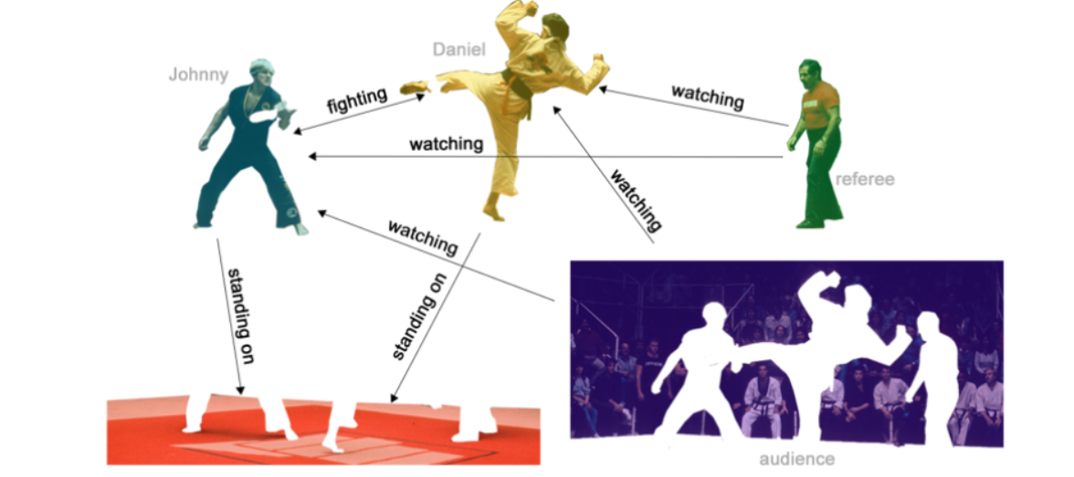
3、数据集：Zachary's karate club network.

该图描述了一个空手道俱乐部会员的社交关系，以34名会员作为节点，如果两位会员在俱乐部之外仍保持社交关系，则在节点间增加一条边。
每个节点具有一个34维的特征向量，一共有78条边。
在收集数据的过程中，管理人员 John A 和 教练 Mr. Hi（化名）之间产生了冲突，会员们选择了站队，一半会员跟随 Mr. Hi 成立了新俱乐部，剩下一半会员找了新教练或退出了俱乐部。

4、 PyTorch Geometric

• 这个就是咱们的核心了，说白了就是这里实现了各种图神经网络中的方法
• 咱们直接调用就可以了：PyTorch Geometric (PyG) library

数据集介绍

• 可以直接参考其API：https://pytorch-geometric.readthedocs.io/en/latest/modules/datasets.html#torch_geometric.datasets.KarateClub

from torch_geometric.datasets import KarateClub

dataset = KarateClub()
print(f'Dataset: {dataset}:')
print('======================')
print(f'Number of graphs: {len(dataset)}')
print(f'Number of features: {dataset.num_features}')
print(f'Number of classes: {dataset.num_classes}')

Dataset: KarateClub():
======================
Number of graphs: 1
Number of features: 34
Number of classes: 4

data = dataset[0]  # Get the first graph object.

print(data)

Data(x=[34, 34], edge_index=[2, 156], y=[34], train_mask=[34])

• 图的表示用Data格式（说明可以点击）

5、edge_index

• edge_index：表示图的连接关系（start,end两个序列）
• node features：每个点的特征
• node labels：每个点的标签
• train_mask：有的节点木有标签（用来表示哪些节点要计算损失）

edge_index = data.edge_index
print(edge_index)

tensor([[ 0,  0,  0,  0,  0,  0,  0,  0,  0,  0,  0,  0,  0,  0,  0,  0,  1,  1,
          1,  1,  1,  1,  1,  1,  1,  2,  2,  2,  2,  2,  2,  2,  2,  2,  2,  3,
          3,  3,  3,  3,  3,  4,  4,  4,  5,  5,  5,  5,  6,  6,  6,  6,  7,  7,
          7,  7,  8,  8,  8,  8,  8,  9,  9, 10, 10, 10, 11, 12, 12, 13, 13, 13,
         13, 13, 14, 14, 15, 15, 16, 16, 17, 17, 18, 18, 19, 19, 19, 20, 20, 21,
         21, 22, 22, 23, 23, 23, 23, 23, 24, 24, 24, 25, 25, 25, 26, 26, 27, 27,
         27, 27, 28, 28, 28, 29, 29, 29, 29, 30, 30, 30, 30, 31, 31, 31, 31, 31,
         31, 32, 32, 32, 32, 32, 32, 32, 32, 32, 32, 32, 32, 33, 33, 33, 33, 33,
         33, 33, 33, 33, 33, 33, 33, 33, 33, 33, 33, 33],
        [ 1,  2,  3,  4,  5,  6,  7,  8, 10, 11, 12, 13, 17, 19, 21, 31,  0,  2,
          3,  7, 13, 17, 19, 21, 30,  0,  1,  3,  7,  8,  9, 13, 27, 28, 32,  0,
          1,  2,  7, 12, 13,  0,  6, 10,  0,  6, 10, 16,  0,  4,  5, 16,  0,  1,
          2,  3,  0,  2, 30, 32, 33,  2, 33,  0,  4,  5,  0,  0,  3,  0,  1,  2,
          3, 33, 32, 33, 32, 33,  5,  6,  0,  1, 32, 33,  0,  1, 33, 32, 33,  0,
          1, 32, 33, 25, 27, 29, 32, 33, 25, 27, 31, 23, 24, 31, 29, 33,  2, 23,
         24, 33,  2, 31, 33, 23, 26, 32, 33,  1,  8, 32, 33,  0, 24, 25, 28, 32,
         33,  2,  8, 14, 15, 18, 20, 22, 23, 29, 30, 31, 33,  8,  9, 13, 14, 15,
         18, 19, 20, 22, 23, 26, 27, 28, 29, 30, 31, 32]])

inde是稀疏表示的，并不是n*n的邻接矩阵

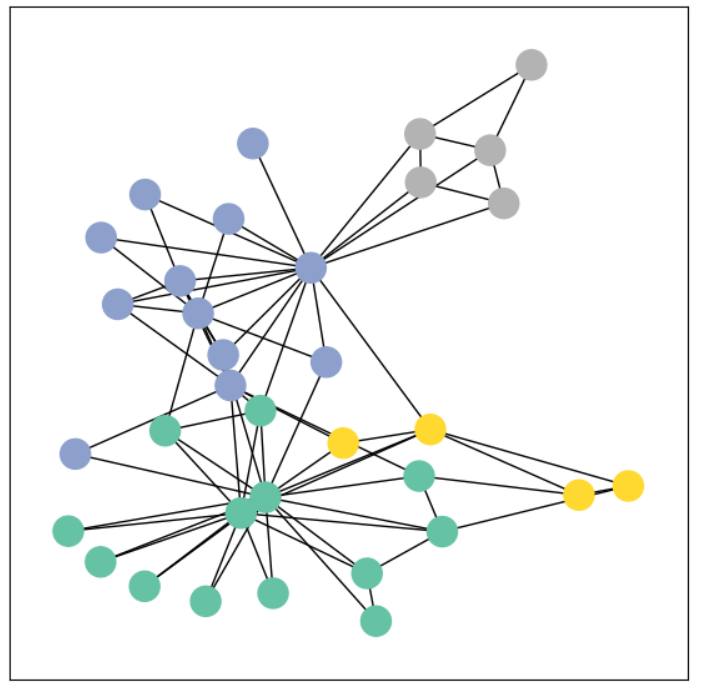
使用networkx可视化展示

from torch_geometric.utils import to_networkx

G = to_networkx(data, to_undirected=True)
visualize_graph(G, color=data.y)

6、Graph Neural Networks 网络定义：

• GCN layer (Kipf et al. (2017)) 定义如下：

\[\mathbf{x}_v^{(\ell + 1)} = \mathbf{W}^{(\ell + 1)} \sum_{w \in \mathcal{N}(v) \, \cup \, \{ v \}} \frac{1}{c_{w,v}} \cdot \mathbf{x}_w^{(\ell)} \]

• PyG 文档 GCNConv

import torch
from torch.nn import Linear
from torch_geometric.nn import GCNConv


class GCN(torch.nn.Module):
    def __init__(self):
        super().__init__()
        torch.manual_seed(1234)
        self.conv1 = GCNConv(dataset.num_features, 4) # 只需定义好输入特征和输出特征即可
        self.conv2 = GCNConv(4, 4)
        self.conv3 = GCNConv(4, 2)
        self.classifier = Linear(2, dataset.num_classes)

    def forward(self, x, edge_index):
        h = self.conv1(x, edge_index) # 输入特征与邻接矩阵（注意格式，上面那种）
        h = h.tanh()
        h = self.conv2(h, edge_index)
        h = h.tanh()
        h = self.conv3(h, edge_index)
        h = h.tanh()  
        
        # 分类层
        out = self.classifier(h)

        return out, h

model = GCN()
print(model)

GCN(
  (conv1): GCNConv(34, 4)
  (conv2): GCNConv(4, 4)
  (conv3): GCNConv(4, 2)
  (classifier): Linear(in_features=2, out_features=4, bias=True)
)

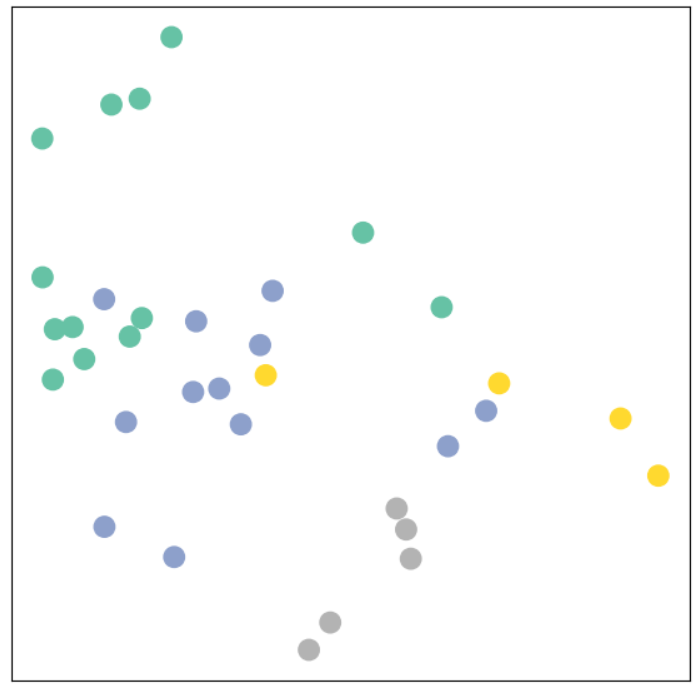
输出特征展示

• 最后不是输出了两维特征嘛，画出来看看长啥样
• 但是，但是，现在咱们的模型还木有开始训练。。。

model = GCN()

_, h = model(data.x, data.edge_index)
print(f'Embedding shape: {list(h.shape)}')

visualize_embedding(h, color=data.y)

Embedding shape: [34, 2]

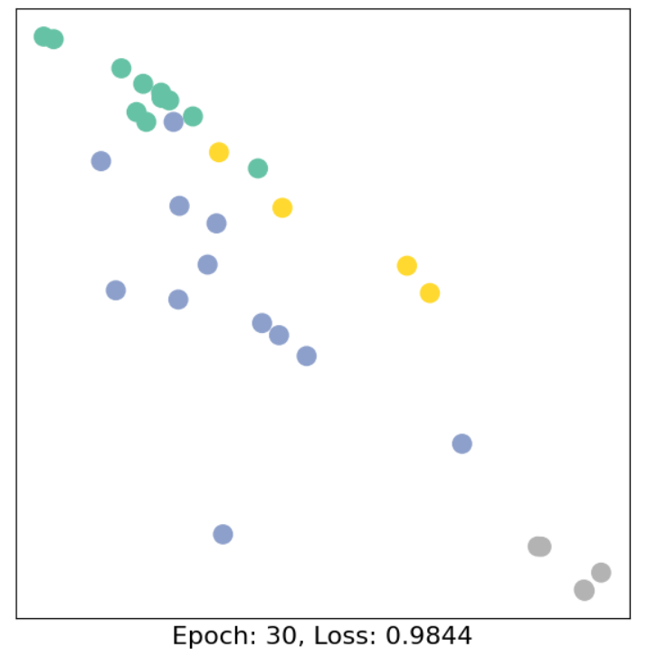
7、训练模型(semi-supervised)

import time

model = GCN()
criterion = torch.nn.CrossEntropyLoss()  # Define loss criterion.
optimizer = torch.optim.Adam(model.parameters(), lr=0.01)  # Define optimizer.

def train(data):
    optimizer.zero_grad()  
    out, h = model(data.x, data.edge_index) #h是两维向量，主要是为了咱们画个图 
    loss = criterion(out[data.train_mask], data.y[data.train_mask])  # semi-supervised
    loss.backward()  
    optimizer.step()  
    return loss, h

for epoch in range(40):
    loss, h = train(data)
    if epoch % 10 == 0:
        visualize_embedding(h, color=data.y, epoch=epoch, loss=loss)
        time.sleep(0.3)