tensorflow(二十三)：函数优化

一、函数

 

 

 

 

 

 绘图代码

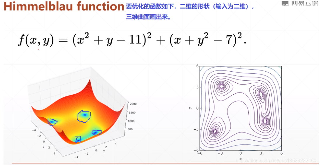
import tensorflow as tf
import numpy as np
from mpl_toolkits.mplot3d import Axes3D
import matplotlib.pyplot as plt
import os

os.environ['TF_CPP_MIN_LOG_LEVEL'] = '2'


def himelblau(x):
    return (x[0]**2 + x[1] -11)**2 +(x[0] + x[1]**2 - 7)**2

x = np.arange(-6, 6, 0.1)
y = np.arange(-6, 6, 0.1)
print("x,y range: ", x.shape, y.shape)
X, Y = np.meshgrid(x, y)
print("X,Y maps: ", X.shape, Y.shape)
Z = himelblau([X, Y])

fig = plt.figure('himelblau')
ax = fig.gca(projection='3d')
ax.plot_surface(X, Y, Z)
ax.view_init(60, -30)
ax.set_xlabel('x')
ax.set_ylabel('y')
plt.show()

想深入理解绘图请参考文档：python笔记：numpy中mgrid的用法

二、梯度下降

 

 

 

注意下面两点：

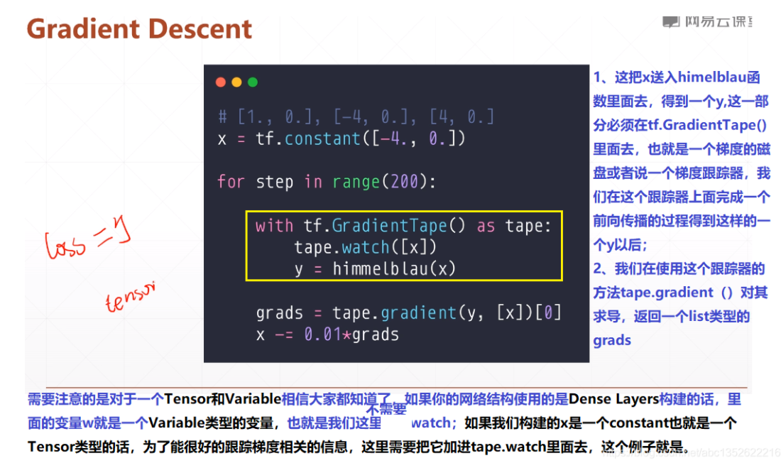
对于一个Tensor和Variable类型相信大家都知道了，如果你的网络结构使用的是Dense Layers构建的，里面的变量w, b类型就是Variable类型的变量， 也就是不需要watch；如果我们构建的x是一个constant也就是一个Tenosr类型的话，为了更好的跟踪梯度的相关信息，这里需要把它加进tape.watch里面去，这个例子就是。
tf.GradientTape里面默认只会跟踪tf.Variable()类型。如果类型不是这个的话。这里为tf.tensor,tf.Variable是tf.tensor的一种特殊类型。因此简单的包装一下，在tensor类型外面包一个Variable类型。

import tensorflow as tf
import numpy as np
from mpl_toolkits.mplot3d import Axes3D
import matplotlib.pyplot as plt
import os

os.environ['TF_CPP_MIN_LOG_LEVEL'] = '2'


def himelblau(x):
    return (x[0]**2 + x[1] -11)**2 +(x[0] + x[1]**2 - 7)**2

x = np.arange(-6, 6, 0.1)
y = np.arange(-6, 6, 0.1)
print("x,y range: ", x.shape, y.shape)
X, Y = np.meshgrid(x, y)
print("X,Y maps: ", X.shape, Y.shape)
Z = himelblau([X, Y])

fig = plt.figure('himelblau')
ax = fig.gca(projection='3d')
ax.plot_surface(X, Y, Z)
ax.view_init(60, -30)
ax.set_xlabel('x')
ax.set_ylabel('y')
plt.show()

# [1., 0.], [-4, 0.], [4, 0.]
x = tf.constant([-4., 0.]) #初始点的坐标（x, y）


for step in range(200):  #迭代200次。
    with tf.GradientTape() as tape:
        tape.watch([x])
        y = himelblau(x)

    grads = tape.gradient(y, [x])[0]
    #print(grads)
    x -=0.01*grads


    if step % 20 ==0:
        print('step {0}: x = {1}, f(x) = {2}'.format(step, x.numpy(),y.numpy()))

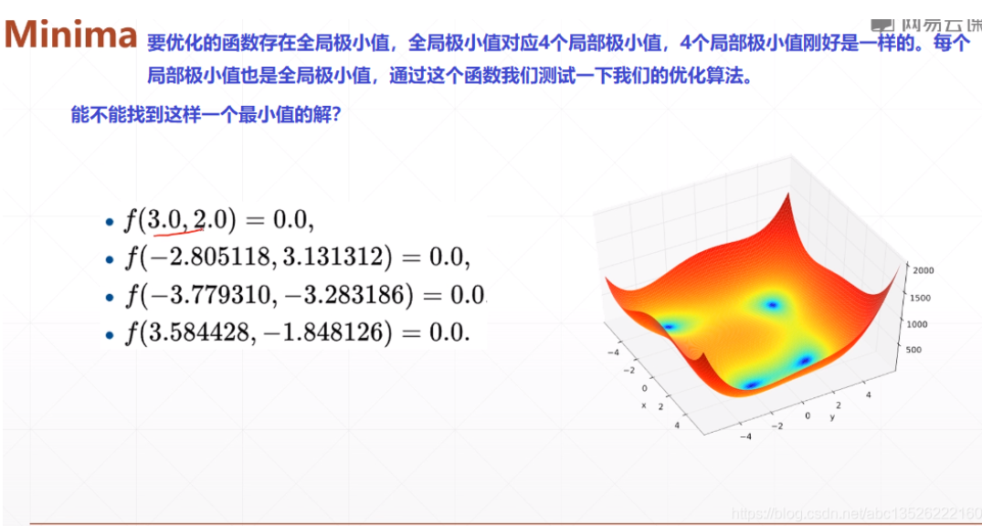
可以很快发现找到最小值，使f(x)=0；对比刚才的标准解，改变初始坐标，会有惊奇的发现。
我们改变初始坐标：通过梯度下降法搜索的时候，会按照不同的路径搜索（下图的2个坐标），同时也可以知道，梯度下降的任何一个超参数都会影响我们的最终的结果，所以我们在做deep learning的时候，需要非常的细心，要想取得很好的解，每一个细节我们都需要注意。