实验二:逻辑回归算法实验
【实验目的】
理解逻辑回归算法原理,掌握逻辑回归算法框架;
理解逻辑回归的sigmoid函数;
理解逻辑回归的损失函数;
针对特定应用场景及数据,能应用逻辑回归算法解决实际分类问题。
【实验内容】
1.根据给定的数据集,编写python代码完成逻辑回归算法程序,实现如下功能:
建立一个逻辑回归模型来预测一个学生是否会被大学录取。假设您是大学部门的管理员,您想根据申请人的两次考试成绩来确定他们的入学机会。您有来自以前申请人的历史数据,可以用作逻辑回归的训练集。对于每个培训示例,都有申请人的两次考试成绩和录取决定。您的任务是建立一个分类模型,根据这两门考试的分数估计申请人被录取的概率。
算法步骤与要求:
(1)读取数据;(2)绘制数据观察数据分布情况;(3)编写sigmoid函数代码;(4)编写逻辑回归代价函数代码;(5)编写梯度函数代码;(6)编写寻找最优化参数代码(可使用scipy.opt.fmin_tnc()函数);(7)编写模型评估(预测)代码,输出预测准确率;(8)寻找决策边界,画出决策边界直线图。
2. 针对iris数据集,应用sklearn库的逻辑回归算法进行类别预测。
要求:
(1)使用seaborn库进行数据可视化;(2)将iri数据集分为训练集和测试集(两者比例为8:2)进行三分类训练和预测;(3)输出分类结果的混淆矩阵。
【实验报告要求】
对照实验内容,撰写实验过程、算法及测试结果;
代码规范化:命名规则、注释;
实验报告中需要显示并说明涉及的数学原理公式;
查阅文献,讨论逻辑回归算法的应用场景;
实验内容及结果
1.根据给定的数据集,编写python代码完成逻辑回归算法程序
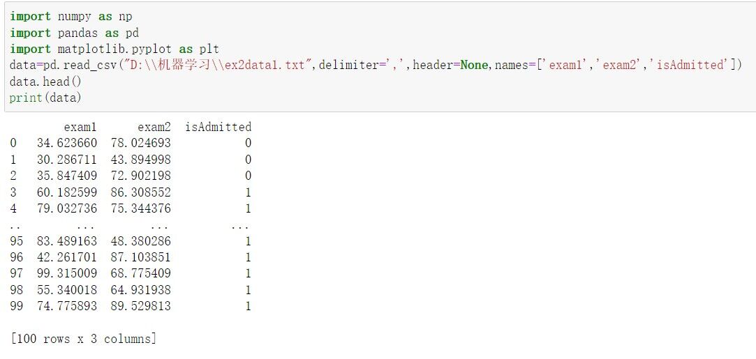
(1)读取数据
#导入包和数据
import numpy as np
import pandas as pd
import matplotlib.pyplot as plt
data=pd.read_csv("D:\\机器学习\\ex2data1.txt",delimiter=',',header=None,names=['exam1','exam2','isAdmitted'])
data.head()
print(data)
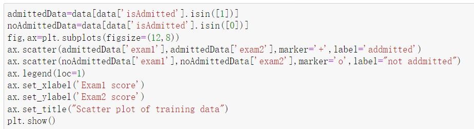
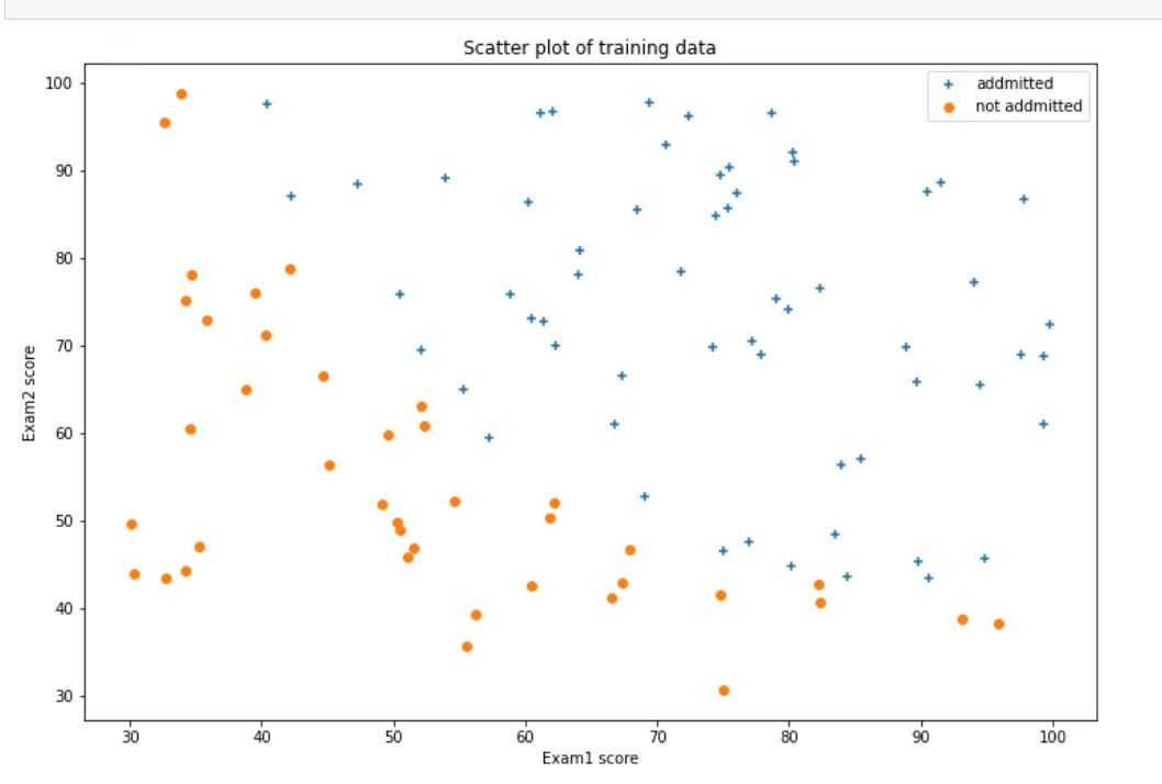
(2)绘制数据观察数据分布情况
#绘制数据观察数据分布情况
admittedData=data[data['isAdmitted'].isin([1])]
noAdmittedData=data[data['isAdmitted'].isin([0])]
fig,ax=plt.subplots(figsize=(12,8))
ax.scatter(admittedData['exam1'],admittedData['exam2'],marker='+',label='addmitted')
ax.scatter(noAdmittedData['exam1'],noAdmittedData['exam2'],marker='o',label="not addmitted")#描绘散点图
ax.legend(loc=1)
ax.set_xlabel('Exam1 score')
ax.set_ylabel('Exam2 score')
ax.set_title("Scatter plot of training data")#添加x轴,y轴,主题名字
plt.show()
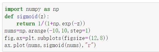
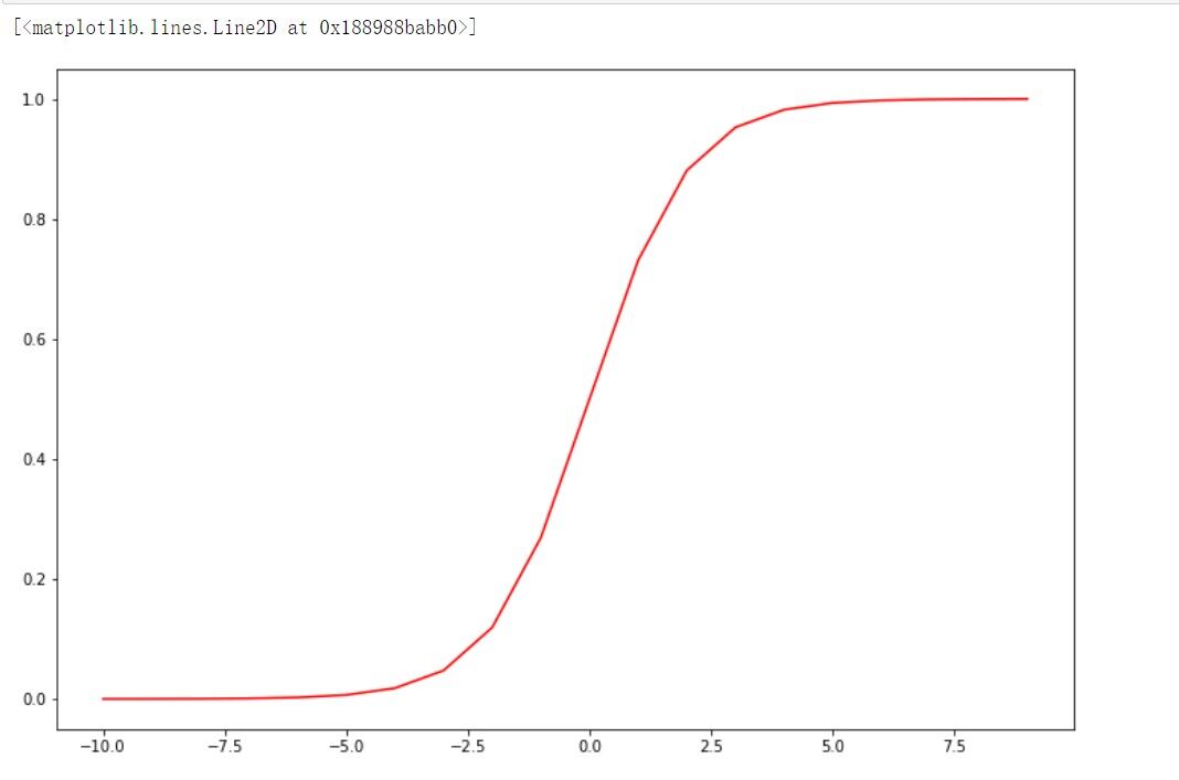
(3)编写sigmoid函数
#sigmoid函数
import numpy as np
def sigmoid(z):
    return 1/(1+np.exp(-z))
nums=np.arange(-10,10,step=1)
fig,ax=plt.subplots(figsize=(12,8))#设置画布大小
ax.plot(nums,sigmoid(nums),"r")
(4)编写逻辑回归代价函数
#逻辑回归代价函数
data.insert(0, 'ones',1)
loc=data.shape[1]
X=np.array(data.iloc[:,0:loc-1])
Y=np.array(data.iloc[:,loc-1:loc])
theta=np.zeros(X.shape[1])
X.shape,Y.shape,theta.shape

def computeCost(theta,X,Y):
    theta = np.matrix(theta)
    h=sigmoid(np.dot(X,(theta.T)))
    a=np.multiply(-Y,np.log(h))
    b=np.multiply((1-Y),np.log(1-h))
    return np.sum(a-b)/len(X)
computeCost(theta,X,Y)

(5)编写梯度函数
#梯度函数
def gradient(theta,X,Y):
    theta = np.matrix(theta) #theta转化为矩阵
    h=sigmoid(np.dot(X,(theta.T)))
    grad=np.dot(((h-Y).T),X)/len(X)
    return np.array(grad).flatten()

gradient(theta,X,Y)

(6)寻找最优化参数
#寻找最优化参数
import scipy.optimize as opt
result = opt.fmin_tnc(func=computeCost, x0=theta, fprime=gradient, args=(X, Y))
print(result)
theta=result[0]

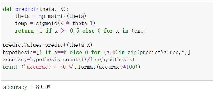
(7)模型评估(预测)输出预测准确率
#模型评估(预测)输出预测准确率
def predict(theta, X):
    theta = np.matrix(theta)
    temp = sigmoid(X * theta.T)
    return [1 if x >= 0.5 else 0 for x in temp] #预测结果>=0.5为1,否则为0

predictValues=predict(theta,X)
hypothesis=[1 if a==b else 0 for (a,b)in zip(predictValues,Y)]
accuracy=hypothesis.count(1)/len(hypothesis)
print ('accuracy = {0}%'.format(accuracy*100))
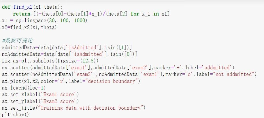
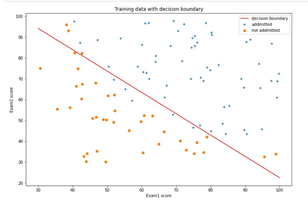
(8)寻找决策边界,画出决策边界直线图
#寻找决策边界,画出决策边界直线图
def find_x2(x1,theta):
    return [(-theta[0]-theta[1]*x_1)/theta[2] for x_1 in x1]
x1 = np.linspace(30, 100, 1000)
x2=find_x2(x1,theta)

#数据可视化
admittedData=data[data['isAdmitted'].isin([1])]
noAdmittedData=data[data['isAdmitted'].isin([0])]
fig,ax=plt.subplots(figsize=(12,8))
ax.scatter(admittedData['exam1'],admittedData['exam2'],marker='+',label='addmitted')
ax.scatter(noAdmittedData['exam2'],noAdmittedData['exam1'],marker='o',label="not addmitted")
ax.plot(x1,x2,color='r',label="decision boundary")
ax.legend(loc=1)
ax.set_xlabel('Exam1 score')
ax.set_ylabel('Exam2 score')
ax.set_title("Training data with decision boundary")
plt.show()
2. 针对iris数据集,应用sklearn库的逻辑回归算法进行类别预测
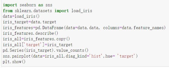
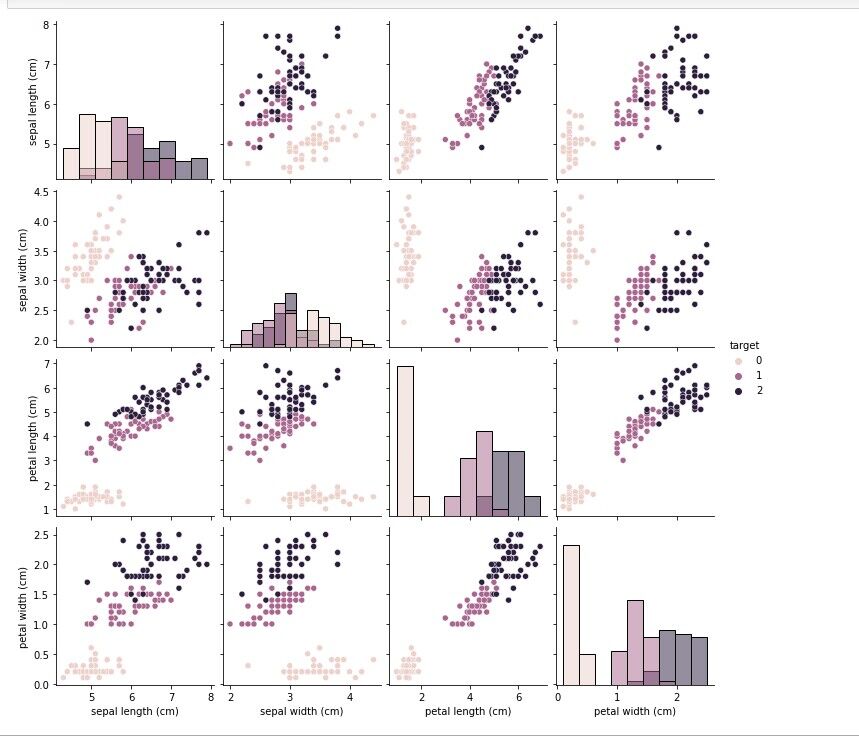
(1)使用seaborn库进行数据可视化
import seaborn as sns
from sklearn.datasets import load_iris
data=load_iris()
iris_target=data.target
iris_features=pd.DataFrame(data=data.data, columns=data.feature_names)
iris_features.describe()
iris_all=iris_features.copy()
iris_all['target']=iris_target
pd.Series(iris_target).value_counts()
sns.pairplot(data=iris_all,diag_kind='hist',hue= 'target')
plt.show()
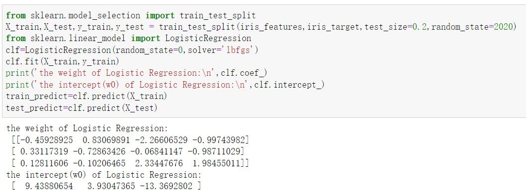
(2)将iri数据集分为训练集和测试集(两者比例为8:2)进行三分类训练和预测
from sklearn.model_selection import train_test_split
X_train,X_test,y_train,y_test = train_test_split(iris_features,iris_target,test_size=0.2,random_state=2020)
from sklearn.linear_model import LogisticRegression
clf=LogisticRegression(random_state=0,solver='lbfgs')
clf.fit(X_train,y_train)
print('the weight of Logistic Regression:\n',clf.coef_)
print('the intercept(w0) of Logistic Regression:\n',clf.intercept_)
train_predict=clf.predict(X_train)
test_predict=clf.predict(X_test)
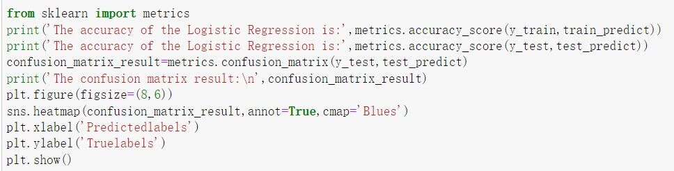
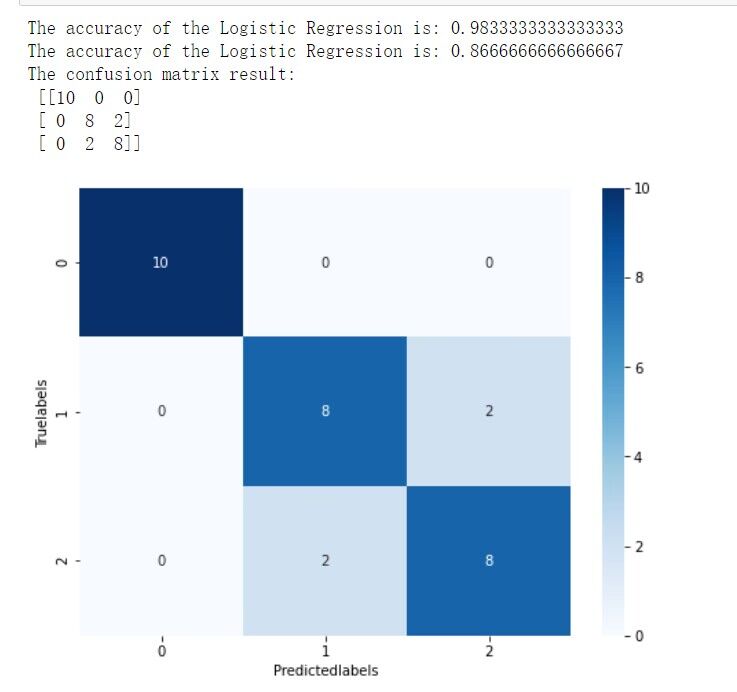
(3)输出分类结果的混淆矩阵
from sklearn import metrics
print('The accuracy of the Logistic Regression is:',metrics.accuracy_score(y_train,train_predict))
print('The accuracy of the Logistic Regression is:',metrics.accuracy_score(y_test,test_predict))
confusion_matrix_result=metrics.confusion_matrix(y_test,test_predict)
print('The confusion matrix result:\n',confusion_matrix_result)
plt.figure(figsize=(8,6))
sns.heatmap(confusion_matrix_result,annot=True,cmap='Blues')
plt.xlabel('Predictedlabels')
plt.ylabel('Truelabels')
plt.show()
3.函数
sigmoid函数
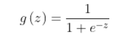
sigmoid函数,会把线性回归的结果映射到【0,1】之间,假设0.5为阈值,默认会把小于0.5的为0,大于0.5的为1
代价函数
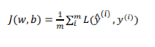
损失函数是在单个训练样本中定义的,它衡量的是算法在单个训练样本中表现如何,为了衡量算法在全部训练样本上的表现如何,我们需要定义一个算法的代价函数,算法的代价函数是对m个样本的损失函数求和然后除以m

在只考虑单个样本的情况,单个样本的代价函数定义如下:其中a是逻辑回归的输出,y是样本的标签值

4.逻辑回归算法的应用场景
应用:
用于分类:适合做很多分类算法的基础组件
用于预测:预测事件发生的概率(输出)
用于分析:单一因素对某一个事件发生的影响因素分析(特征参数值)