Image Scaling using Deep Convolutional Neural Networks
Image Scaling using Deep Convolutional Neural Networks
This past summer I interned at Flipboard in Palo Alto, California. I worked on machine learning based problems, one of which was Image Upscaling. This post will show some preliminary results, discuss our model and its possible applications to Flipboard’s products.
High quality and a print-like finish play a key role in Flipboard’s design language. We want users to enjoy a consistent and beautiful experience throughout all of Flipboard’s content, as if they had a custom print magazine in hand. Providing this experience consistently is difficult. Different factors, such as image quality, deeply affect the overall quality of the presented content. Image quality varies greatly depending on the image’s source. This varying image quality is especially apparent in magazines that display images across the whole page in a full bleed format.
When we display images on either the web or mobile devices they must be above a certain threshold to display well. If we receive a large image on our web product we can create breathtaking full bleed sections.

Lower resolution images introduce pixelation, over smoothing and artifacts when scaled above 100%. This is especially apparent in a full bleed presentation as seen below. This severely reduces the quality of presentation in our products.

What is the cause of this? In general, when we need an image of size X that is required to be of size Y it must be run through a scaling algorithm. This algorithm performs a mathematical operation to scale the image pixels to the desired size Y. Some of the possible algorithms are bicubic, bilinear, and nearest-neighbor interpolation. Many of the algorithms listed above perform an interpolation between pixel values to create a transition. These algorithms use the surrounding pixels to guess what the missing values should be in the new image. The problem in the case of scaling the image to a larger size is when there are too many ‘new’ values to be filled in the image. These algorithms try to make “guesses” of what the new values should be but this introduces errors in the process which leads to noise, haloing, and artifacts.
Before we go any further I would like to give a high level introduction to both the traditional and convolutional flavours of Neural Networks. If you have a good grasp of them feel free to skip ahead to next section. Following the introduction to Neural Networks there is a preliminary results section, discussion of the model architectures, design decisions, and applications.
Note: Smaller nuances of Neural Networks will not be covered in the introduction.
Neural Networks
Neural Networks are an amazing type model that is able to learn from given data. They have a large breadth of applications and have enjoyed a recent resurgence in popularity in many domains such as computer vision, audio recognition, and natural language processing. Some recent feats includecaptioning images, playing Atari, aiding self-driving cars, and language translation.
Neural Networks exist in different configurations, such as convolutional andrecurrent, that are each good at different types of tasks. Learning ‘modes’ also exist: supervised and unsupervised; we will only focus on supervised learning.
Supervised learning is described as a network that is trained on both an input and an output. This ‘mode’ is used to predict new outputs given an input. An example of this would be training a network on thousands of pictures of cats and dogs which have been manually labelled and then asking, on a new picture, is this a cat or dog?
On a structural level a Neural Network is a feedforward graph where each of the nodes, known as units, performs a nonlinear operation on the incoming inputs. Each of the inputs has a weight that the network is able to learn through an algorithm known as backpropagation.

Source: Wikipedia
The structure of a Neural Network is flexible and based on the task at hand. We are free to customize our network by selecting attributes such as: the number of hidden layers (blue nodes above), number of units per layer, number of connections per unit etc. These attributes known as hyperparameters describe our model’s structure and behaviour. Selecting these parameters correctly is critical to achieving high performance. Hyperparameters are usually chosen through random grid search, optimization algorithms (bayesian and gradient based), or simple trial and error.
As mentioned previously the units within a network perform a mathematical operation on the inputs. We can take a closer look by calculating a simple numerical example involving a single unit with a handful of inputs.

The unit above takes three inputs: x1,x2,x3 and a scalar bias term b (not shown). Each of these inputs has weightings that are referred to as w1,w2, and w3. The weights express the importance of the incoming input. The bias term allows us to offset our weighted value to the left or right. For this example we will use the Rectified Linear (ReL) function as the units mathematical operation, more formally known as an activation function, expressed as:
The gist of this activation function is any input value below zero is considered as zero and anything above remains the same. It has an output range of [0,∞]. Other activation functions can also be used such as the sigmoid, hyperbolic tangent, and maxout.
So how do we calculate an output value? To do so we need to compute f(WTx+b). The first step is to compute the vector product between transpose W and x, defined as WTx. Our bias value is then added to this result before finally being passed through our activation function.
To make this example a little more concrete we will use some random numbers. Say we have the following vectors corresponding to our weights, inputs, and scalar bias value:
Going step by step we calculate the result of WTx:
Then our bias value is added WTx+b:
We then take this quantity and pass it through our activation function f(x):
As per our function definition we see that if x is greater than zero we will get the value of x out, which in this case is 3.54.
Why is this exciting? Well, in terms of a single unit, it is not too exciting. As it stands, we can tweak the weights and bias value to model only the most basic of functions. Our little example lacks ‘expressive power’. In order to increase our ‘expressive power’ we can chain and link units together to form larger networks as seen below.

The equations for the network above, where Wfrom,to is the weight from one unit to another, is as follows:
z1 is the the same expression we calculated earlier! See how we have chained them together to create a more complicated network? We are applying the same calculation over and over. We use the output from a previous layer of units to compute the next. The values are propagated through the network until they arrive at the final layer. We call this process forward propagation. But this process is of little use to us if we need to change the output of our network as it makes no adjustments to the weights and biases.
To update the weights and biases of our network we will use an algorithm known as backpropagation. We will focus on a supervised approach where our network is given pairs of data: input x and the desired output y. In order to usebackpropagation in this supervised manner we need to quantify our network’s performance. We must define an error that compares the result of forward propagation through our network, y^(our estimated value), against the desired value y.
This comparison between values is formally known as a cost function. It can be defined however you want but for this post we will use the mean squared error function:
This function gives us a magnitude of error. If our network was given randomly initialized weights and biases the output will be far from the desired y value, causing a large output from EMSE.
Backpropagation takes this magnitude and propagates it from the back of the network to the front adjusting the weights and biases along the way. The amount of adjustment to each weight and bias can be thought of as its contribution to the error and is calculated through gradient descent. This algorithm seeks to minimize the error function above by changing the weights and biases.
The general process to train a Neural Network, given an input vector x and the expected output y, is as follows:
- Perform a step of forward propagation through the network with input vector x. We will calculate an output y^.
- Calculate the error with our error function. EMSE(x,y)=1n|y^(x)−y|2.
- Backpropagate the errors through our network updating the weights and biases.
The above steps are repeated over and over with different xand y pairs until the weights and biases of our network give us the minimum error possible! We are minimizing the EMSE function.
Convolutional Neural Networks
If you have been paying attention to recent tech articles you will most likely have heard of Neural Networks breaking the state-of-the-art in several domains. These breakthroughs are due in a small part to convolutional Neural Networks.
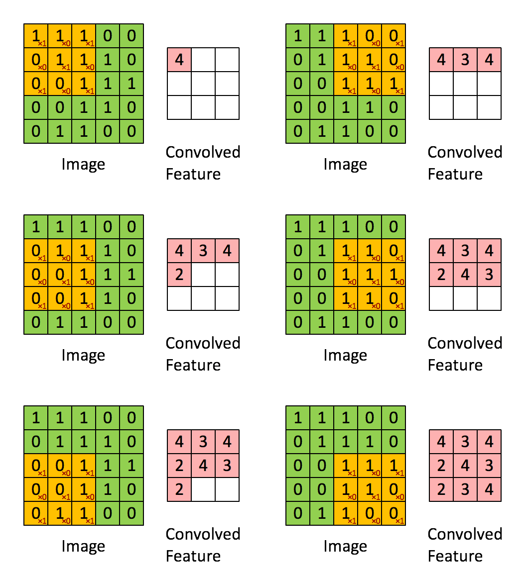
Convolutional Neural Networks (convnets) are a slightly different flavour of the typical feed-forward Neural Network. Convnets take some biological inspiration from the visual cortex, which contains small regions of cells that are sensitive to subregions of the visual field. This is referred to as a receptive field. We can mimic this small subfield by learning weights in the form of matrices, referred to as ‘kernels’; which, like their biologically inspired counterparts, are sensitive to similar subregions of an image. We now require a way to express the similarity between our kernel and the subregion. Since the convolution operation essentially returns a measure of ‘similarity’ between two signals we can happily pass a learned kernel, along with a subregion of the image, through this operation and have a measure of similarity returned back!
Below is an animation of a kernel, in yellow, being convolved over an image, in green, with the result of the operation on the right in red.

Source: Feature extraction using convolution from Stanford Deep Learning
To illustrate this let’s run a very simple square kernel which detects directional edges over an image. The weights of our kernel:
Applying the convolutional operation using our kernel, several times over the left image, we get the image on the right:

Source: Edge Detection with Matrix Convolution
So why is this useful? In the context of Neural Networks several reasons exist:
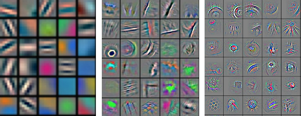
This allows us to extract information from the right image above. The kernels inform us of the presence and location of directional edges. When used in a Neural Network we can learn the appropriate weight settings of the kernels to extract out basic features such as edges, gradients and blurs. If the network is deep with enough convolutional layers it will start learning feature combinations off of the previous layers. The simple building blocks of edges, gradients, and blurs become things like eyes, noses, and hair in later layers!

Source: Yann Lecun “ICML 2013 tutorial on Deep Learning”
Traditionally if we wanted to do work in the image or audio domains we would have to perform feature generation using other algorithms that would preprocess our data into a usable form. This would then allow our machine learning algorithm of choice to make sense of the incoming data. This process is tedious and fragile. By applying a convolutional frontend to our networks we are able to let the algorithm, with minimal preprocessing of the data on our side, to create the features that work best for that specific domain and situation. The network does feature extraction on its own. The learned features of the network work better than most of the algorithmically and hand engineered features.
Image Scaling using Convolutional Neural Networks
Below is a collection of preliminary results that were produced from the model. The left image is the original ‘high’ resolution. This is the ground truth and what we would hope to get with perfect reconstruction. We scale this original down by a factor of 2x and send it through either a bicubic scaling algorithm or the model. The results are in the center and right positions respectively.


The major differences can be seen between the hairline, eyebrows, and skin on the cheek and forehead.


The model does a good job along the hard edges on the balcony and on the sun tanning beds in the foreground.


This one is difficult to see at first glance. The finer details, such as the hair along the side of the ear and on the inside of the ear are present in the model.


No image related work is complete unless Lenna is included in some way. Observe the sharpness of the feathers, noise, lips, and eyes. The pattern on the hat also shows up better in the model output.


The major differences between the versions are the tree leaves, shadow shapes and tree textures.
Architecture
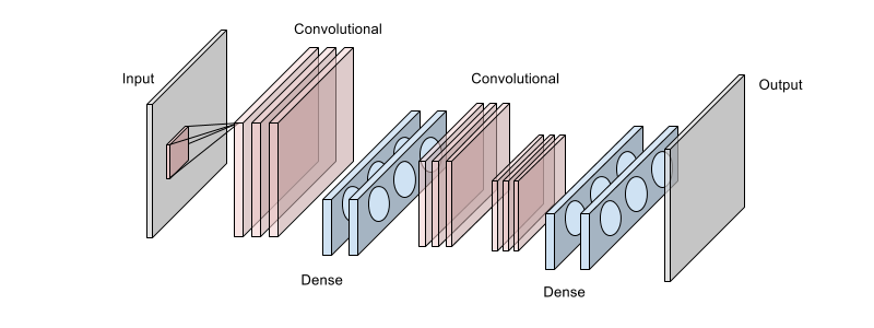
Below is one of the architectures used, the primary goal is to double the number of pixels taken in from the image. The architecture is a 8 layer Neural Network composed of three convolutional layers, each shown as stacked pinkish blocks, and four fully connected layers colored in blue. Each layer uses the rectified linear activation function. There is a final dense layer with linear Gaussian units which is not shown below.

A small section of the input image is ingested through the first convolutional layer. This image was collected from the larger image using a square sliding window. The first convolutional contains the largest number of filter maps. The outputs are ‘reprojected’ into a higher dimensionality through the first two dense fully-connected layers. Their output is further processed by the next two convolutional layers. Features from the two convolutional layers are then fed into a series of fully-connected layers. The final output image is calculated by a linear Gaussian layer.
No pooling operations are used after any of the convolutional layers. While pooling is useful for classification tasks, where invariance to input is important, the location of features detected by each kernel is important. Pooling also discards too much useful information which is the opposite of what is needed for this use case.
The weights were all initialized using the Xavier initialization suggested by Glorot & Benigo and was then slightly tweaked during hyperparameter optimzation. This is defined as 2nin+nout and was sampled from a normal distribution. The biases were all initialized to zero.
Dataset
The network was trained on a large dataset of approximately 3 million samples. The dataset images used natural images including those of animals and outdoor scenes. Some images needed to be filtered out of this set as they included illustrations of animals or text. As each image was of varying size and quality a constraint in the form of a pixel count was added to focus on images which contained a total pixel count of 640,000 and up.
Each sample within the dataset is a low and high resolution image pair. The low resolution image, the ‘x’ input, was created by downscaling a high resolution image by a certain factor. While the desired output, ‘y’, was of the original high resolution image. Very mild noise and distortions were added to the input data. The data was normalized to have zero mean by calculating the global mean and to unit variance by dividing through by the standard deviation of the dataset.
The dataset was divided into subsets of training, testing, and validation; following a 80%, 10%, and 10% split respectively.
Regularization
Max Norm
Max norm constraints enforce an absolute upper bound on the weight vectors magnitude for every unit in that layer which stops the network’s weights from ‘exploding’ if the gradient update is too large. Max norm constraints are used in all layers except the final linear Gaussian layer. An aggressive magnitude was used in all of the convolutional layers while the other layers’ magnitudes were much more lax.
L2
L2 regularization penalizes the network for using large weight vectors, W. This is set by the parameter λ and is known as the regularization strength. It is added to the cost function as the term 12λW2. The optimization algorithm tries to keep the weights small while minimizing the cost function as before. The convolutional layers and first two densely connected layers have mild regularization applied and the other densely connected layers use a stronger value.
Dropout
Dropout randomly ‘drops’ units from a layer on each training step, creating ‘sub-architectures’ within the model. It can be viewed as a type of sampling of a smaller network within a larger network. Only the weights of the included units are updated, which makes sure the network does not become too reliant on a few units. This process of removing units happens over and over between runs, so the units being included change. The convolutional layers all have a high inclusion probability of almost 1.0 while the last two fully connected layers include about half the units.

Training
The model was trained using Stochastic Gradient descent in batch sizes of 250 over the entire training set for ~250 epochs. A highish batchsize was used to smooth out the updates and make better use of the GPUs while still getting some benefit from perturbations of smaller batches.
The network is trained to minimize a mean square error function. A learning rate scale was used on all weights and biases. The formula for the weights (per layer) was 1−12nintotal2 where ni is the current layer position and ntotal is the total number of layers. This scaled the learning rate which helped the earlier layers converge. All the biases had a learning rate multiplier of 2.0. Nesterov momentum was used with an initial value of 0.15 and increased to 0.7 over 45 epochs.
Amazon g2.2xlarge EC2 instances were used to train the network with NVIDIA’s cuDNN library added in to speed up training. Training the final model took approximately 19 hours.
Hyperparameters
The majority of the hyperparameters were selected using an inhouse hyperparameter optimization library that works over clusters of Amazon g2.2xlarge instances. This was performed using a portion of the training dataset and the validation dataset. The process took roughly ~4 weeks and evaluated ~500 different configurations.
Variations
Some things that did not work out well while working on this problem:
- Used a larger batch size of 1000, this worked well, but ran up against local minima quickly. The jitter provided by a smaller batch was useful to bounce out of these minimas.
- Used a small convolutional network, this was alright but did not generalize as well as the larger convolutional network.
- Tried to use the weight initialization formula suggested by He et al. : 2n. Unfortunately this caused the network to sputter around and it failed to learn. Might be this specific configuration as many people have successfully used it.
- Used the same amount of L2 regularization on all layers, it worked much better to vary the L2 regularization based on which layers started saturating or were clamped against max normal constraints.
- Used pooling on the layers. Lost too much information between layers, images turned out grainy and poor looking.
The biggest lesson learned dealing with these larger networks is how important it is to getting the weight initializations right. I feel this aspect, after a few other hyperparameters are chosen, has the largest impact on how well your model will train. It is a good idea to spend time researching the different initialization techniques to understand the impact each has on your model. There are many papers and machine learning libraries out there with different initialization schemes from which you can easily learn.
Applications
Our goal was not to remove or replace the need for other upscaling algorithms, such as bicubic upscaling, but to try to improve quality using different technology and avenues. Our primary use case was to scale lower resolution images up when no higher resolution images are available. This happens occasionally across our platforms.
Besides the primary use case of still images this technique can be applied to different media formats such as GIFs. The GIF could be split into its separate frames, then scaled up, and then repackaged.
The final use case that we thought of was saving bandwidth. A smaller image could be sent to the client which would run a client side version of this model to gain a larger image. This could be accomplished using a custom solution or one of the javascript implementations of neural networks available such asConvNetJS.
Further steps
We feel this problem space has a lot of potential and there are many things to try, including some wild ideas, such as:
- Larger filter sizes in the convolutional layers.
- Try more layers and data.
- Try different color channel formats instead of RGB.
- Try using hundreds of filters in the first convolutional layer, sample from them using dropout with a very small inclusion probability and try tweaking the learning rate of the layer.
- Ditch the fully connected layers and try using all convolutional layers.
- Curious if distillation would work with this problem. Might help create a lighter version to run on client devices easily.
- Look into how small/large we can make the network before the quality starts degrading.
Conclusion
Pursuing high fidelity presentation is difficult. As with any endeavor, it takes an exceeding amount of effort to squeeze out those final few percentage points of quality. We are constantly reflecting on our product to see where those percentage points can come from, even if they don’t seem obvious or possible at first. While this wont have its place everywhere within our product, we feel it was a good cursory step forward to improving quality.
I hope you enjoyed reading through this post and have taken something interesting away with it. I would like to thank everyone at Flipboard for an outstanding internship experience. I have learnt a lot, met many awesome people, and gained invaluable experience in the process.
If machine learning, large datasets, and working with great people on interesting projects excites you then feel free to apply, we are hiring!
Feel free to follow me on twitter @normantasfi
Special thanks to Charles, Emil, Anh, Mike Klaas, and Michael Johnston for suggestions and edits throughout the process. Shoutout to Greg for always making time to help with server setups and questions.


 浙公网安备 33010602011771号