NEURAL NETWORKS, PART 1: BACKGROUND
NEURAL NETWORKS, PART 1: BACKGROUND
Artificial neural networks (NN for short) are practical, elegant, and mathematically fascinating models for machine learning. They are inspired by the central nervous systems of humans and animals – smaller processing units (neurons) are connected together to form a complex network that is capable of learning and adapting.
The idea of such neural networks is not new. McCulloch-Pitts (1943) described binary threshold neurons already back in 1940’s. Rosenblatt (1958) popularised the use of perceptrons, a specific type of neurons, as very flexible tools for performing a variety of tasks. The rise of neural networks was halted after Minsky and Papert (1969) published a book about the capabilities of perceptrons, and mathematically proved that they can’t really do very much. This result was quickly generalised to all neural networks, whereas it actually applied only to a specific type of perceptrons, leading to neural networks being disregarded as a viable machine learning method.
In recent years, however, the neural network has made an impressive comeback. Research in the area has become much more active, and neural networks have been found to be more than capable learners, breaking state-of-the-art results on a wide variety of tasks. This has been substantially helped by developments in computing hardware, allowing us to train very large complex networks in reasonable time. In order to learn more about neural networks, we must first understand the concept of vector space, and this is where we’ll start.
A vector space is a space where we can represent the position of a specific point or object as a vector (a sequence of numbers). You’re probably familiar with 2 or 3-dimensional coordinate systems, but we can easily extend this to much higher dimensions (think hundreds or thousands). However, it’s quite difficult to imagine a 1000-dimensional space, so we’ll stick to 2-dimensional illustations.
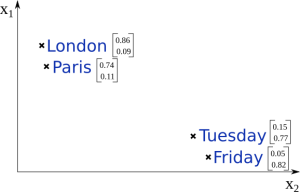
In the graph below, we have placed 4 objects in a 2-dimensional space, and each of them has a 2-dimensional vector that represents their position in this space. For machine learning and classification we make the assumption that similar objects have similar coordinates and are therefore positioned close to each other. This is true in our example, as cities are positioned in the upper left corner, and days-of-the-week are positioned a bit further in the lower right corner.
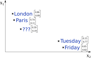
Let’s say we now get a new object (see image below) and all we know are its coordinates. What do you think, is this object a city or a day-of-the-week? It’s probably a city, because it is positioned much closer to other existing cities we already know about.
This is the kind of reasoning that machine learning tries to perform. Our example was very simple, but this problem gets more difficult when dealing with thousands of dimensions and millions of noisy datapoints.
In a traditional machine learning context these vectors are given as input to the classifier, both at training and testing time. However, there exist methods of representation learning where these vectors are learned automatically, together with the model.
Now that we know about vector spaces, it’s time to look at how the neuron works.
References
- McCulloch, Warren S., and Walter Pitts. “A logical calculus of the ideas immanent in nervous activity.” The Bulletin of Mathematical Biophysics 5.4 (1943): 115-133.
- Minsky, Marvin, and Papert Seymour. “Perceptrons.” (1969).
- Rosenblatt, Frank. “The perceptron: a probabilistic model for information storage and organization in the brain.” Psychological review 65.6 (1958): 386.


 浙公网安备 33010602011771号