Numerical Optimization: Understanding L-BFGS

http://aria42.com/blog/2014/12/understanding-lbfgs/

Numerical optimization is at the core of much of machine learning. Once you’ve defined your model and have a dataset ready, estimating the parameters of your model typically boils down to minimizing some multivariate function 

f(x), where the input x is in some high-dimensional space and corresponds to model parameters. In other words, if you solve:

x∗=argminxf(x)

then x∗ is the ‘best’ choice for model parameters according to how you’ve set your objective.1

In this post, I’ll focus on the motivation for the L-BFGS algorithm for unconstrained function minimization, which is very popular for ML problems where ‘batch’ optimization makes sense. For larger problems, online methods based around stochastic gradient descent have gained popularity, since they require fewer passes over data to converge. In a later post, I might cover some of these techniques, including my personal favorite AdaDelta.

Note: Throughout the post, I’ll assume you remember multivariable calculus. So if you don’t recall what a gradient or Hessian is, you’ll want to bone up first.

Newton’s Method

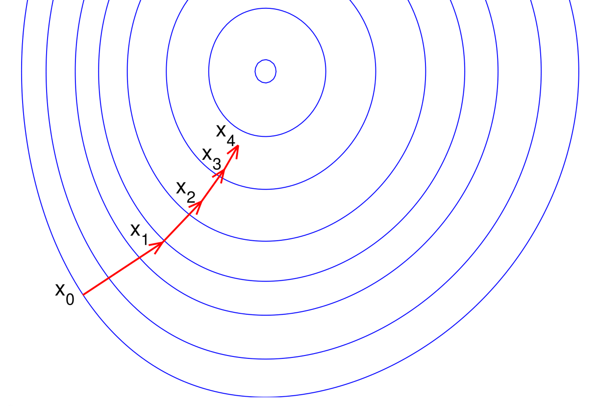
Most numerical optimization procedures are iterative algorithms which consider a sequence of ‘guesses’ xn which ultimately converge to x∗ the true global minimizer of f. Suppose, we have an estimate xn and we want our next estimate xn+1 to have the property that f(xn+1)<f(xn).

Newton’s method is centered around a quadratic approximation of f for points near xn. Assuming that f is twice-differentiable, we can use a quadratic approximation of f for points ‘near’ a fixed pointx using a Taylor expansion:

f(x+Δx)≈f(x)+ΔxT∇f(x)+12ΔxT(∇2f(x))Δx

where ∇f(x) and ∇2f(x) are the gradient and Hessian of f at the point xn. This approximation holds in the limit as ||Δx||→0. This is a generalization of the single-dimensional Taylor polynomial expansion you might remember from Calculus.

In order to simplify much of the notation, we’re going to think of our iterative algorithm of producing a sequence of such quadratic approximations hn. Without loss of generality, we can write xn+1=xn+Δx and re-write the above equation,

hn(Δx)=f(xn)+ΔxTgn+12ΔxTHnΔx

where gn and Hn represent the gradient and Hessian of f at xn.

We want to choose Δx to minimize this local quadratic approximation of f at xn. Differentiating with respect to Δx above yields:

∂hn(Δx)∂Δx=gn+HnΔx

Recall that any Δx which yields ∂hn(Δx)∂Δx=0 is a local extrema of hn(⋅). If we assume that Hn ispostive semi-definite (psd) then we know this Δx is also a global minimum for hn(⋅). Solving for Δx:2

Δx=−H−1ngn

This suggests H−1ngn as a good direction to move xn towards. In practice, we set xn+1=xn−α(H−1ngn) for a value of α where f(xn+1) is ‘sufficiently’ smaller than f(xn).

Iterative Algorithm

The above suggests an iterative algorithm:

NewtonRaphson(f,x0):For n=0,1,… (until converged):Compute gn and H−1n for xnd=H−1ngnα=minα≥0f(xn−αd)xn+1←xn−αd

The computation of the α step-size can use any number of line search algorithms. The simplest of these is backtracking line search, where you simply try smaller and smaller values of α until the function value is ‘small enough’.

In terms of software engineering, we can treat NewtonRaphson as a blackbox for any twice-differentiable function which satisfies the Java interface:

public interface TwiceDifferentiableFunction {
  // compute f(x)
  public double valueAt(double[] x);

  // compute grad f(x)
  public double[] gradientAt(double[] x);

  // compute inverse hessian H^-1
  public double[][] inverseHessian(double[] x);
}

With quite a bit of tedious math, you can prove that for a convex function, the above procedure will converge to a unique global minimizer x∗, regardless of the choice of x0. For non-convex functions that arise in ML (almost all latent variable models or deep nets), the procedure still works but is only guranteed to converge to a local minimum. In practice, for non-convex optimization, users need to pay more attention to initialization and other algorithm details.

Huge Hessians

The central issue with NewtonRaphson is that we need to be able to compute the inverse Hessian matrix.3 Note that for ML applications, the dimensionality of the input to f typically corresponds to model parameters. It’s not unusual to have hundreds of millions of parameters or in some vision applications even billions of parameters. For these reasons, computing the hessian or its inverse is often impractical. For many functions, the hessian may not even be analytically computable, let along representable.

Because of these reasons, NewtonRaphson is rarely used in practice to optimize functions corresponding to large problems. Luckily, the above algorithm can still work even if H−1n doesn’t correspond to the exact inverse hessian at xn, but is instead a good approximation.

Quasi-Newton

Suppose that instead of requiring H−1n be the inverse hessian at xn, we think of it as an approximation of this information. We can generalize NewtonRaphson to take a QuasiUpdate policy which is responsible for producing a sequence of H−1n.

QuasiNewton(f,x0,H−10,QuasiUpdate):For n=0,1,… (until converged):// Compute search direction and step-size d=H−1ngnα←minα≥0f(xn−αd)xn+1←xn−αd// Store the input and gradient deltas gn+1←∇f(xn+1)sn+1←xn+1−xnyn+1←gn+1−gn// Update inverse hessian H−1n+1←QuasiUpdate(H−1n,sn+1,yn+1)

We’ve assumed that QuasiUpdate only requires the former inverse hessian estimate as well tas the input and gradient differences (sn and yn respectively). Note that if QuasiUpdate just returns∇2f(xn+1), we recover exact NewtonRaphson.

In terms of software, we can blackbox optimize an arbitrary differentiable function (with no need to be able to compute a second derivative) using QuasiNewton assuming we get a quasi-newton approximation update policy. In Java this might look like this,

public interface DifferentiableFunction {
  // compute f(x)
  public double valueAt(double[] x);

  // compute grad f(x)
  public double[] gradientAt(double[] x);  
}

public interface QuasiNewtonApproximation {
  // update the H^{-1} estimate (using x_{n+1}-x_n and grad_{n+1}-grad_n)
  public void update(double[] deltaX, double[] deltaGrad);

  // H^{-1} (direction) using the current H^{-1} estimate
  public double[] inverseHessianMultiply(double[] direction);
}

Note that the only use we have of the hessian is via it’s product with the gradient direction. This will become useful for the L-BFGS algorithm described below, since we don’t need to represent the Hessian approximation in memory. If you want to see these abstractions in action, here’s a link to aJava 8 and golang implementation I’ve written.

Behave like a Hessian

What form should QuasiUpdate take? Well, if we have QuasiUpdate always return the identity matrix (ignoring its inputs), then this corresponds to simple gradient descent, since the search direction is always ∇fn. While this actually yields a valid procedure which will converge to x∗ for convex f, intuitively this choice of QuasiUpdate isn’t attempting to capture second-order information about f.

Let’s think about our choice of Hn as an approximation for f near xn:

hn(d)=f(xn)+dTgn+12dTHnd

Secant Condition

A good property for hn(d) is that its gradient agrees with f at xn and xn−1. In other words, we’d like to ensure:

∇hn(xn)∇hn(xn−1)=gn=gn−1

Using both of the equations above:

∇hn(xn)−∇hn(xn−1)=gn−gn−1

Using the gradient of hn+1(⋅) and canceling terms we get

Hn(xn−xn−1)=(gn−gn−1)

This yields the so-called “secant conditions” which ensures that Hn+1 behaves like the Hessian at least for the diference (xn−xn−1). Assuming Hn is invertible (which is true if it is psd), then multiplying both sides by H−1n yields

H−1nyn=sn

where yn+1 is the difference in gradients and sn+1 is the difference in inputs.

Symmetric

Recall that the a hessian represents the matrix of 2nd order partial derivatives: H(i,j)=∂f/∂xi∂xj. The hessian is symmetric since the order of differentiation doesn’t matter.

The BFGS Update

Intuitively, we want Hn to satisfy the two conditions above:

• Secant condition holds for sn and yn
• Hn is symmetric

Given the two conditions above, we’d like to take the most conservative change relative to Hn−1. This is reminiscent of the MIRA update, where we have conditions on any good solution but all other things equal, want the ‘smallest’ change.

minH−1s.t. ∥H−1−H−1n−1∥2H−1yn=snH−1 is symmetric 

The norm used here ∥⋅∥ is the weighted frobenius norm.4 The solution to this optimization problem is given by

H−1n+1=(I−ρnynsTn)H−1n(I−ρnsnyTn)+ρnsnsTn

where ρn=(yTnsn)−1. Proving this is relatively involved and mostly symbol crunching. I don’t know of any intuitive way to derive this unfortunately.

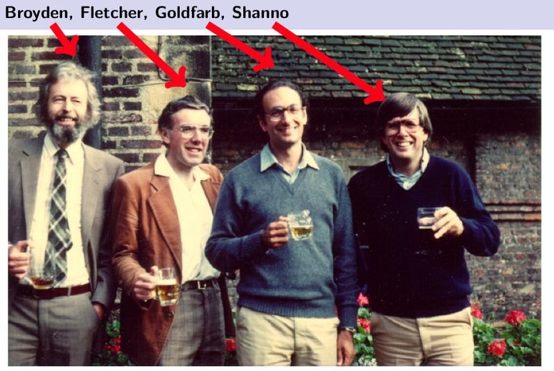
This update is known as the Broyden–Fletcher–Goldfarb–Shanno (BFGS) update, named after the original authors. Some things worth noting about this update:

• H−1n+1 is positive semi-definite (psd) when H−1n is. Assuming our initial guess of H0 is psd, it follows by induction each inverse Hessian estimate is as well. Since we can choose any H−10we want, including the I matrix, this is easy to ensure.

• The above also specifies a recurrence relationship between H−1n+1 and H−1n. We only need the history of sn and yn to re-construct H−1n.

The last point is significant since it will yield a procedural algorithm for computing H−1nd, for a direction d, without ever forming the H−1n matrix. Repeatedly applying the recurrence above we have

BFGSMultiply(H−10,{sk},{yk},d):r←d// Compute right productfor i=n,…,1:αi←ρisTirr←r−αiyi// Compute centerr←H−10r// Compute left productfor i=1,…,n:β←ρiyTirr←r+(αn−i+1−β)sireturn r

Since the only use for H−1n is via the product H−1ngn, we only need the above procedure to use the BFGS approximation in QuasiNewton.

L-BFGS: BFGS on a memory budget

The BFGS quasi-newton approximation has the benefit of not requiring us to be able to analytically compute the Hessian of a function. However, we still must maintain a history of the sn and ynvectors for each iteration. Since one of the core-concerns of the NewtonRaphson algorithm were the memory requirements associated with maintaining an Hessian, the BFGS Quasi-Newton algorithm doesn’t address that since our memory use can grow without bound.

The L-BFGS algorithm, named for limited BFGS, simply truncates the BFGSMultiply update to use the last m input differences and gradient differences. This means, we only need to store sn,sn−1,…,sn−m−1 and yn,yn−1,…,yn−m−1 to compute the update. The center product can still use any symmetric psd matrix H−10, which can also depend on any {sk} or {yk}.

L-BFGS variants

There are lots of variants of L-BFGS which get used in practice. For non-differentiable functions, there is an othant-wise varient which is suitable for training L1 regularized loss.

One of the main reasons to not use L-BFGS is in very large data-settings where an online approach can converge faster. There are in fact online variants of L-BFGS, but to my knowledge, none have consistently out-performed SGD variants (including AdaGrad or AdaDelta) for sufficiently large data sets.

1. This assumes there is a unique global minimizer for f. In practice, in practice unless f is convex, the parameters used are whatever pops out the other side of an iterative algorithm. ↩

2. We know −H−1∇f is a local extrema since the gradient is zero, since the Hessian has positive curvature, we know it’s in fact a local minima. If f is convex, we know the Hessian is always positive semi-definite and we know there is a single unique global minimum. ↩

3. As we’ll see, we really on require being able to multiply by H−1d for a direction d. ↩

4. I’ve intentionally left the weighting matrix W used to weight the norm since you get the same solution under many choices. In particular for any positive-definite W such that Wsn=yn, we get the same solution. ↩