Gradient Descent and Variants - Convergence Rate Summary

Gradient Descent and Variants - Convergence Rate Summary

Credits

• Ben Retch - Berkeley EE227C Convex Optimization Spring 2015
• Moritz Hardt - The Zen of Gradient Descent
• Yu. Nesterov - Efficiency of coordinate descent methods on huge-scale optimization problems
• Peter Richtarik, Martin Takac - Iteration Complexity of Randomized Block-Coordinate Descent Methods for Minimizing a Composite Function

Goals

Summary the convergence rate of various gradient descent variants.

• Gradient Descent
• Gradient Descent with Momentum
• Stochastic Gradient Descent
• Coordinate Gradient Descent

with a focus on the last one.

1. Gradient Descent

1.1. Defining Algorithm

Gradient Descent in 2D. Images Credit: http://vis.supstat.com/2013/03/gradient-descent-algorithm-with-r/

 

 

The goal here is to minimize a convex function f:Rn→R without constraint.

Definition [Convex function] A function f:Rn→R is convex if its domain of f is a convex set, and ∀x,y∈dom(f), we have

f(θx+(1−θ)y)≤θf(x)+(1−θ)f(y)

 

Graphically, it means if we connect two points in the graph of the function to create a linear line, that linear line lies above the function (for those points in between). We often work with a nicer definition of convex function, when it is differentiable, as in

Theorem [First Order Condition] Suppose f is differentiable. Then f is convex iff its domain is convex and

f(y)≥f(x)+∇f(x)T(y−x),∀x,y

 

Graphically, it means the tangent line lies below the function at any point. Finally, we state the second-order condition for completeness.

Theorem [Second Order Condition] Assume that f is twice differentiable, that is, its Hessian exists at each point in the domain of f, which is open. Then f is convex iff its Hessian is positive semidefinite.

Working with general convex function turns out to be very hard, we instead need the following condition

Definition [L-Lipschitz Gradient] f is said to has L-Lipschitz gradient iff

|∇f(x)−∇f(y)|≤L||x−y||

⇔f(y)≤f(x)+∇f(x)T(y−x)+L2||y−x||2

 

Graphically, it means the function is not too convex, it is upperbounded by a quadratic function. Having this condition is necessary in most of the convergence result in gradient descent. Having an additional condition will make life even easier, this condition is stated in

Definition [m Strongly Convex] f is strongly convex with constant m iff

f(y)≥f(x)+∇f(x)T(y−x)+m2||y−x||2

 

Basically, it is the opposite of L-Lipschitz gradient, it means the function is not too flat, it is lowerbounded by some quadratic function. We know that at the minimum, a function f has derivative equal to 0. As such the two L-Lipschitz can be thought of as establishing an upperbound of the change in function values in term of input values. The strongly convex can be thought of as establishing a lowerbound of the change in function values in term of input values.

We are now ready to define the Gradient Descent algorithm:

Algorithm [Gradient Descent] For a stepsize α chosen before hand

• Initialize x0
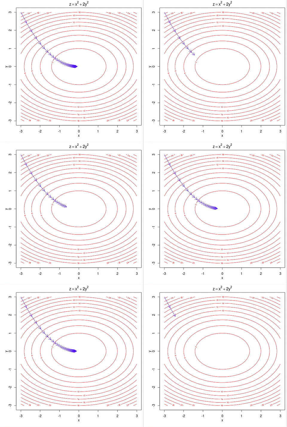
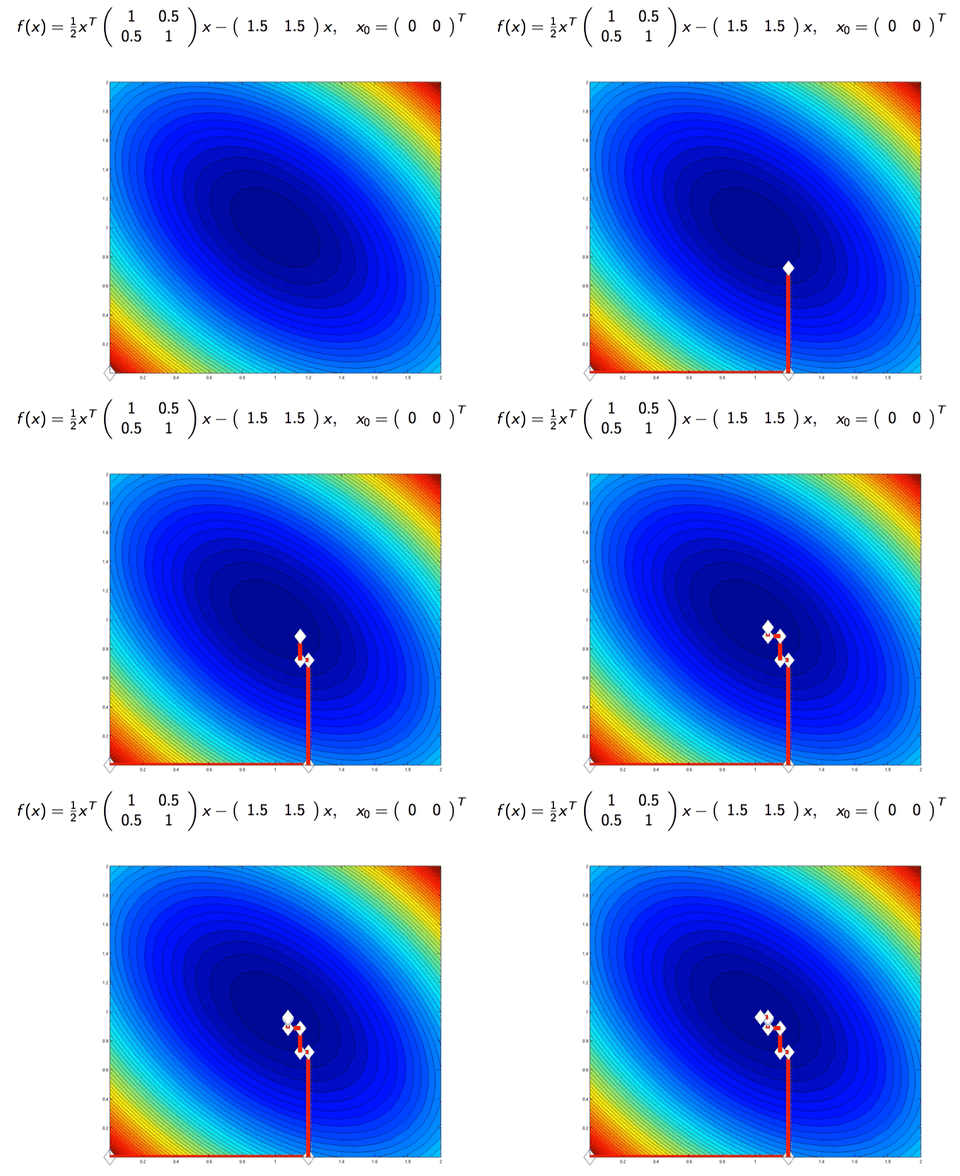
• For k=1,2,..., compute xk+1=xk−α∇f(xk)

Basically, it adjust the xk a little bit in the direction where f decreases the most (the negative gradient direction). In practice, one often choose a variable α instead of a constant α.

1.2. Convergence Rate

Theorem [Rate for L-Lipschitz and m Strongly Convex]. If f is L-Lipschitz and strongly convex with constant m, then the Gradient Descent algorithm converges to the right solution, and picking the stepsize α=1/L we have

f(xk+1)−f(x⋆)≤(1−mL)(f(xk)−f(x⋆))

⇒f(xk+1−f(x⋆)≤(1−mL)k(f(xk)−f(x⋆))

 

We say the function values converges linearly to the optimal value. Also, since we have the relation between function values and input values, we have ||xk−x⋆|| converges linearly to 0. Here x⋆ denotes the solution to the optimization problem. For an error threshold of ϵ, we would need number of iteration in the order of \log \frac{1}{\epsilon} to find a solution within that error threshold.

Theorem [Rate for L-Lipschizt] If f has L-Lipschitz gradient, then

f(xk)−f(x⋆)≤2Lk+1||x0−x⋆||2

 

The convergence rate is not as good, since we are in a more general case. We say the function values converges in log. For an error threshold of ϵ, we now need in the order of 1ϵ iteraions to find a solution within that error threshold. Note that this is much worse than the previous result.

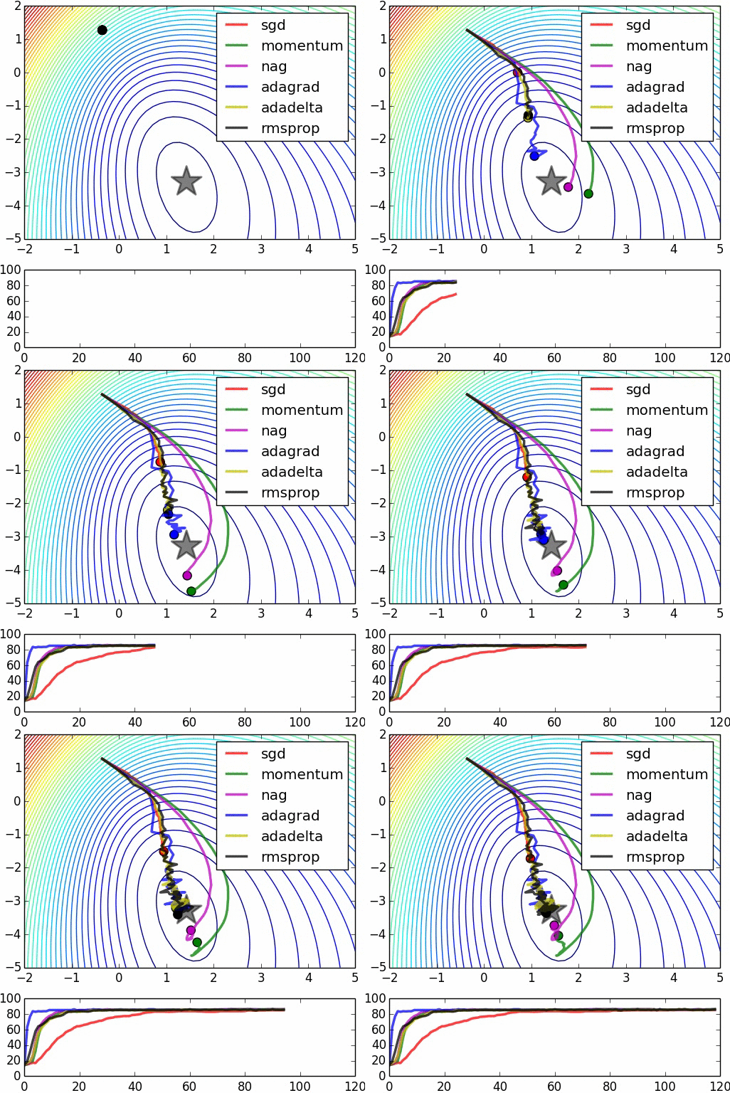
We quickly mention the (Nesterov) momentum method here, basically, each iteration, instead of updating xkalong the direction of gradient, it updates along the weighted average of all the gradient computed so far, with more weight to the recent gradients. I don't think it's quite like that but it is the idea, using the previous computed gradients.

Algorithm [Nesterov Momentum] The update rule for Nesterov method, for constant stepsize α and momentum rate β is

xk+1=xk−α∇f(xk+β(xk−xk−1)+

+β(xk−xk−1)

 

If we were to be careful with the analysis before, for L-Lipschitz gradient and strongly convex function with parameter m, we have the rate of convergence is O(Lmlog1ϵ). With the Nesterov method, we get an improvement to O(Lm−−√log1ϵ). Similarly, for L-Lipschitz gradient, the error rate before was O(Lϵ), now with Nesterov momentum method, we have O(Lϵ−−√). So Nesteve momentum method gives a bit better rate for very little computational cost.

2. Coordinate Descent

2.1. Defining Algorithm

Coordinate Descent in 2D. Images Credit: Martin Takac

 

 

In Machine Learning, we sometimes work with the case where the dimension is too big, or there is too many datapoint. Consider a data matrix X∈Rm×n, if m is too big, one can do Stochastic (Batch) Gradient Descent, which instead of calculating the gradient on all m data points, it approximate the gradient with only b data points, for b is the batch size (for example b=128, while m≈1000000). On the other hand, if n is big, we can upgrade a few of coordinate per iteration, instead of updating the whole n dimension. This is Coordinate descent.

For those problem where calculating coordinate gradient (i.e. partial derivative) is simple, it turns out the the rate for coordinate descent is as good as for typical gradient descent. First let's define the L-Lipschitz condition coordinatewise

Definition [Coordinate-wise Lipschitz gradient] f is L-Lipschitz coordinate-wise with constant Li at coordinate i iff

∥∇f(x+hi)−∇f(x)∥≤Li∥hi∥

for hi is zero everywhere except at coordinate i.

 

We assume our function f is L-Lipschitz coordinate wise with constant Li,i=1,2,...,n. Then the Randomized Coordinate Descent Method is defined as followed:

Algorithm [Randomized Coordinate Descent]

• Pick an initial point x0
• For k=1,2,...
  • pick coordinate i randomly with uniform probability
  • compute xk+1=xk−1Li∇f(x)[i].

Here we introduce the notation ∇f(x)[i] from array notation to say take the ith element of vector ∇f(x). A lot of things can be relaxed from this, for example, the probability can be general not uniform. Instead of doing single coordinate-wise, one can do block coordinate-wise. One can also add a regularization term like ℓ1 (Lasso) or ℓ2 Ridge. See paper by Peter Richtarik and Martin Takac for details. Once can also work with more general norm (in the L-Lipschitz condition). We just state this simple case for simplicity.

2.2. Convergence in Expectation

Theorem [Rate Coordinate Descent with Lipschitz] If we run the above algorithm for coordinate-wise L-Lipschitz gradient, we have

Ek−1f(xk)−f⋆≤2nk+4R2(x0),

for

R(x0)=maxx[maxx⋆∈X⋆∥x−x⋆∥1]:f(x)≤f(x0)

 

So basically, we have the log-convergence rate in expectation, very similar to Gradient Descent. Analogously, the result for strongly convex (globally, not coordinate-wise) is stated in

Theorem [Rate Coordinate Descent with Lipschitz and Strongly Convex m] If we run the above algorithm, we have

Ek−1f(xk)−f⋆≤(1−mn)k(f(x0)−f⋆)

 

Note that here m is the strongly convex parameter, not the number of observation as we used it before. For those of you who are curious, this result and the previous theorem are in Nesterov paper (his Theorem 1 and Theorem 2), applying for the case α=0, which then imply Sα(f)=n.

So basically, we get that for Strongly convex and L-Lipschitz gradient, we also get linear convergence rate in the expectation for Coordinate Descent.

2.3. High Probability Statement

One might also wonder that maybe it works on average, but we only run it once, what is the probability that the result we get from that one time is good. It turns out that our result is good with high probability, as seen in Peter Richtarik, Martin Takac paper. The idea is to used Markov inequality to convert a statement in expectation to a high probability statement. To summary, for a fix confidence interval ρ∈(0,1), if we pick

k≥O(2nϵlogf(x0)−f(x⋆)ϵρ),

we have P[f(xk)−f(x⋆)≤ϵ]≥1−ρ, if the function is coordinate-wise L-Lipschitz gradient.

 

If in addition, we have strongly convex, then the number of iteration needed is only

k≥O(nlog(f(x0)−f(x⋆)ρϵ)).

 

Staring at these high-probability result, we see that the number of iteration needed is almost identical to the case of vanilla Gradient Descent. We have 1/ϵ rate for Lipschitz gradient, and log(1/ϵ) if we have strongly convexity in addition. The rate is however n times slower, because each iteration of Coordinate Descent is approximately n times faster than Gradient Descent (calculating gradient along one coordinate vs calculating gradient along all coordinate). The minor difference is the cost of log1ϵ for the case of only L-Lipschitz can in fact be removed. It is only there when we are optimizing an objective with regularization term (L1 or L2 regularization).

Finally, on a note about momentum for Coordinate Descent, it seems Nesterov recommends not using it, because of the computation complexity for getting the momentum.

3. Stochastic Gradient Descent

Popular optimization algorithms. Images Credit: Daniel Nouri

 

 

It is quite surprised for me that analyzing Stochastic Gradient Descent is much harder than Coordinate Descent. The two algorithms sounds very similar, it is just the former one is vertical, while the later one is horizontal. SGD in fact works very well in practice, it is just proving convergence result is harder. For strongly convex, it seems we only get log convergence rate (as compared to linear in Gradient Descent), as seen in SGD for Machine Learning. For non-strongly convex, we get half the rate. Why??? What is the rate of SGD? To be discovered and written. If you have some ideas please comment.