期末大作业

一、boston房价预测

1. 读取数据集

# 多元线性回归模型
from sklearn.datasets import load_boston
from sklearn.model_selection import train_test_split

 

2. 训练集与测试集划分

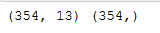
# 多元线性回归模型
data = load_boston()
x_train,x_test,y_train,y_test = train_test_split(data.data,data.target,test_size=0.3)# 划分数据集
print(x_train.shape,y_train.shape)

3. 线性回归模型：建立13个变量与房价之间的预测模型，并检测模型好坏。

# 建立多元线性回归模型
from sklearn.linear_model import LinearRegression
LineR = LinearRegression()
LineR.fit(x_train,y_train)
print('系数',LineR.coef_,'\n截距',LineR.intercept_)

 

4. 多项式回归模型：建立13个变量与房价之间的预测模型，并检测模型好坏。

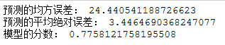
# 检测模型好坏
from sklearn.metrics import regression
y_predict = LineR.predict(x_test)
# 计算模型的预测指标
print("预测的均方误差：",regression.mean_squared_error(y_test,y_predict))
print("预测的平均绝对误差：",regression.mean_absolute_error(y_test,y_predict))
# 打印模型的分数
print("模型的分数：",LineR.score(x_test,y_test))

 

5. 比较线性模型与非线性模型的性能，并说明原因。

非线性模型的模型性能较好，因为它是有很多点连接而成的曲线，对样本的拟合程度较高，而且多项式模型是一条平滑的曲线，更贴合样本点的分布，预测效果误差较小。

二、中文文本分类

分别建立中文文本分类模型，实现对文本的分类。基本步骤如下：

import os
import sys
import numpy as np
from datetime import datetime
path = 'E:\\0369'

# 导入结巴库，并将需要用到的词库加进字典
import jieba
with open(r'E:\\stopsCN.txt',encoding='utf-8') as f:# 导入停用词
    stopwords = f.read().split('\n')

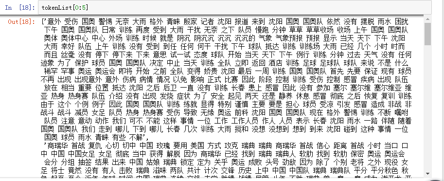
def processing(tokens):
    
    tokens = "".join([char for char in tokens if char.isalpha()])#去掉非字母汉字的字符
    tokens = [token for token in jieba.cut(tokens,cut_all=True) if len(token) >=2]#结巴分词
    tokens = " ".join([token for token in tokens if token not in stopwords])#去掉停用词
    return tokens

tokenList = [] #生成空的文本列表
targetList = [] #类别列表

#用os.walk获取需要的变量，并拼接文件路径再打开每一个文件

#root是当前正在遍历的这个文件夹的本身地址，dirs，files是一个list，
dirs内容是该文件夹中所有的目录的名字，files内容是该文件夹中所有的文件

for root,dirs,files in os.walk(path):

for f in files:
        filePath = os.path.join(root,f)
        with open(filePath,encoding='utf-8') as f:
            content = f.read()

        target = filePath.split('\\')[-2]#分割后的倒数第2个元素#获取新闻类别标签，并处理该新闻
        targetList.append(target)#把各类别追加到干净的tarList = []列表
        tokenList.append(processing(content)) #把预处理过后的文本追加到干净的txtList = []列表

#划分训练集测试集并建立特征向量,为建立模型做准备
from sklearn.feature_extraction.text import TfidfVectorizer
from sklearn.model_selection import train_test_split
from sklearn.naive_bayes import GaussianNB,MultinomialNB
from sklearn.model_selection import cross_val_score
from sklearn.metrics import classification_report
x_train,x_test,y_train,y_test = train_test_split(tokenList,targetList,test_size=0.2,stratify=targetList)#划分训练集测试集

#转化为特征向量，这里选择TfidfVectorizer的方式建立特征向量。不同新闻的词语使用会有较大不同。
vectorizer = TfidfVectorizer()
X_train = vectorizer.fit_transform(x_train)#对部分x训练集数据先拟合
X_test = vectorizer.transform(x_test)#对X测试集进行转化


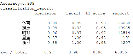
mnb = MultinomialNB()
module = mnb.fit(X_train,y_train)#拟合x,y训练集数据

#进行预测
y_predict = module.predict(X_test)

scores = cross_val_score(mnb,X_test,y_test,cv=5)
print("Accuracy:%.3f"%scores.mean())#输出模型精确度
print("classification_report:\n",classification_report(y_predict,y_test))#输出模型评估报告

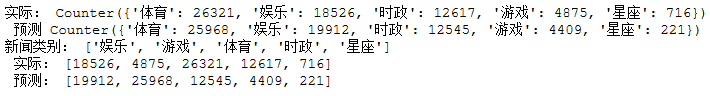
#将预测结果和实际结果进行对比
import collections
import matplotlib.pyplot as plt
from pylab import mpl
mpl.rcParams['font.sans-serif'] = ['FangSong'] #指定默认字体
mpl.rcParams['axes.unicode_minus'] = False #解决保存图像是负号'-'显示为方块的问题

#统计测试集和预测集的各类新闻个数
testCount = collections.Counter(y_test)
predCount = collections.Counter(y_predict)
print('实际：',testCount,'\n', '预测', predCount)

#建立标签列表，实际结果列表，预测结果列表，
nameList = list(testCount.keys()) #各类别名称
testList = list(testCount.values()) #实际结果列表
predictList = list(predCount.values()) #预测结果长度
x = list(range(len(nameList))) #类别长度
print("新闻类别：",nameList,'\n',"实际：",testList,'\n',"预测：",predictList)