机器学习 coursera【week7-9】
week07Support Vector Machines
7.1Large Margin Classification
it is a more cleaner and more powerful way to learn complex non-linear function
start from logistic regression(classification)
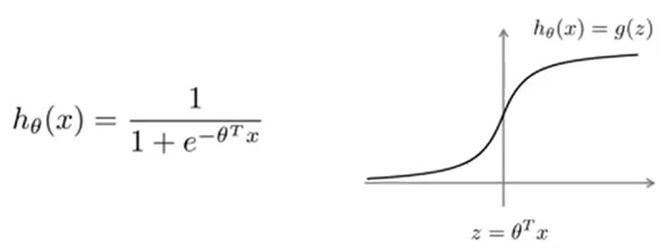
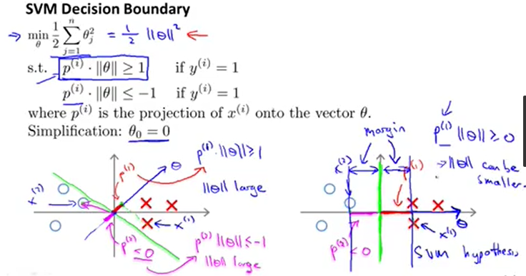
7.2Mathematics behind large margin classification
SVM Decision Boundary: the distance between blue line and green line
7.3Kernels核函数
关于核函数的几个问题:
- 如何选择标记点?
- 如何得到这些标记点?
- 相似度方程是怎么样的?
- 能否用其他核函数来代替高斯核函数?
7.3.1Kernels I
introduction
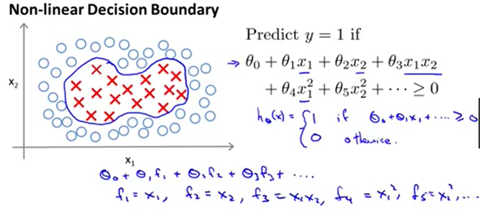
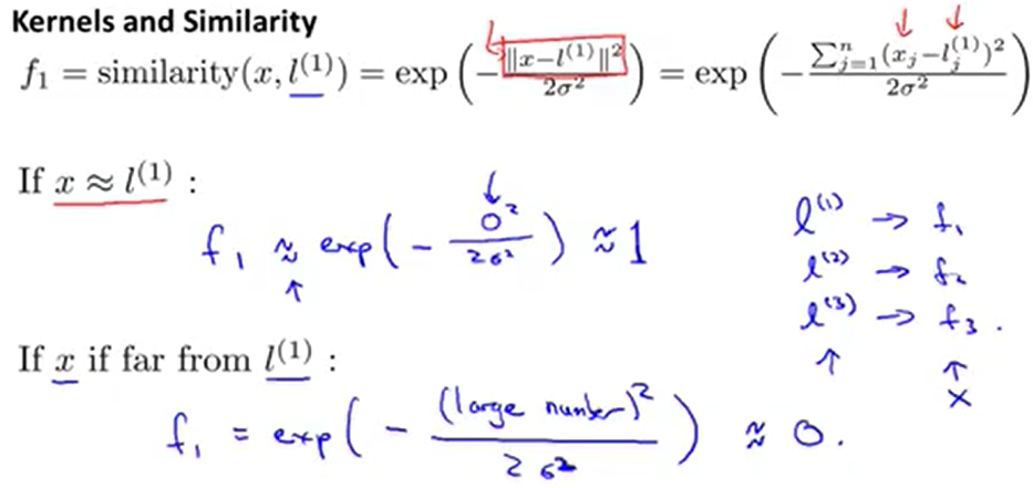
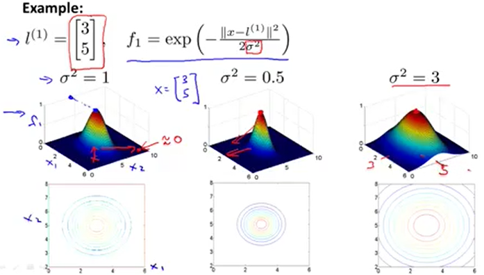
高斯核函数的相似性
不同thegma对应的核函数图像
7.3.1Kernels II
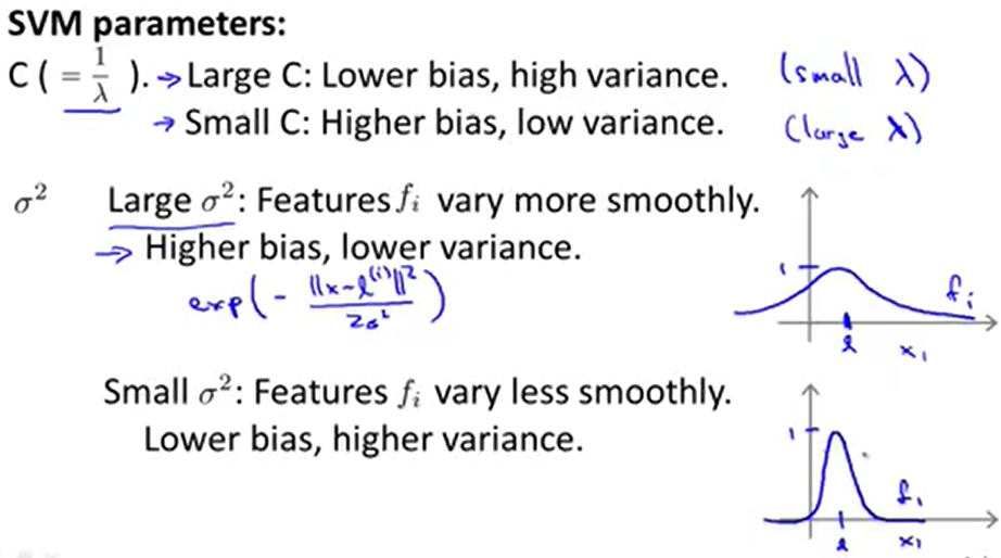
C is equal to 1/lambda, so
large C == small lambda, which means lower bias, high variance and overfitting
small C == large lambda, which means high bias, low variance and underfitting
7.4SVM in practice
SVM software packages like liblinear, libsvm
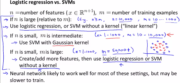
logistic regerssion and SVM
using SVM can find a global minimum to meet the requirement
7.5homework with part1
7.5.1plot the figure with dataset1
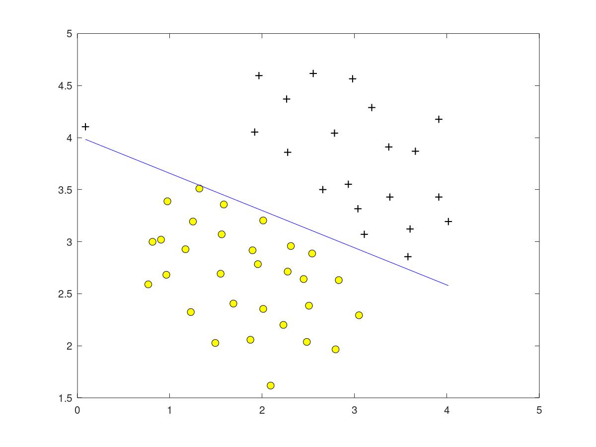
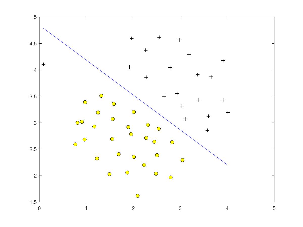
after load the data from ex6data1, we can get a figure which depict all the data
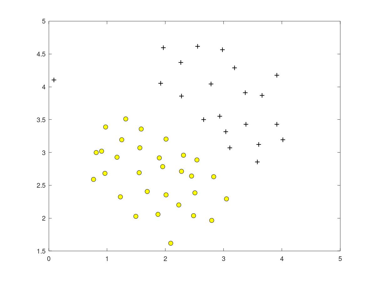
next, train a linear SVM on the dataset and plot the decision boundary learned. so we can get different figure with different lambda.
when the lambda is 1, the figure is like this.
when the lambda is 100, possibly it is likely to overfit.
7.5.2SVM with gaussian kernels
gaussian SVM can be used for the small dataset, however, it is recommended to use other algorithms such as LIBSVM to compute a real problem.
the equation of gaussian kernel

sim = exp((-1)*sum((x1-x2)'*(x1-x2))/(2*sigma*sigma))
notice that the sum could be omitted since there is an addition in the algorithm itself. Originally (x1-x2)'*(x1-x2) is a matrix by 3*3, and by the operation of internal process, it finally is a value.
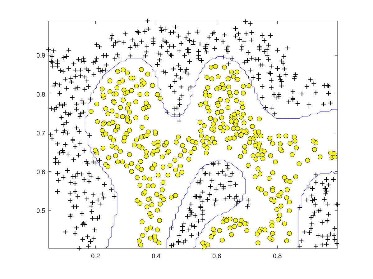
7.5.3plot the data with dataset2(non-linear)

after implementing the gaussian kernel, non-linear decision boundary can be performed.
7.5.3plot the data with dataset3
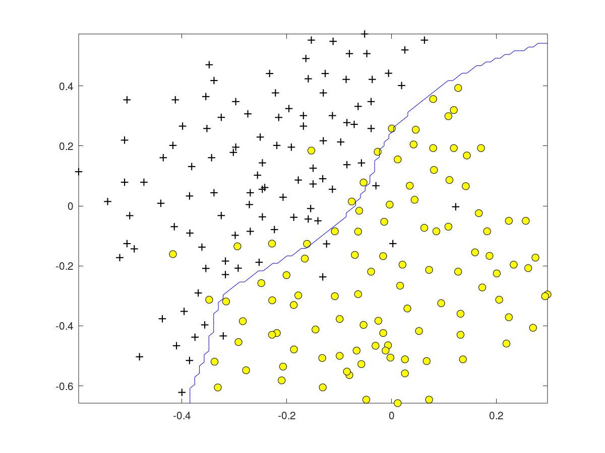
predict the data from cross validation set. after selecting the C and sigma, we could find the optimal parameters of C and sigma to plot the figure of curve.
7.5homework with part2---spam classification
7.5.1how to construct a feature vector from an email
at first, get the email_contents to match the words in the vocabList. Certainly, it is sure to use regularization formula to filter some useless words such as " _","、","!",even some other characters.
after that, introducing the scramp function to match two words whether they are the same or not.
    for  i = 1:length(vocabList) %email_contents
        str1 = str;
        str2 = vocabList{i};
        if strcmp(str1,str2)
            word_indices = [word_indices ; i];
        endif
    endfor
we can get a series of numbers which are word indices.
 86 916 794 1077 883 370 1699 790 1822 1831 883 431 1171 794 1002 1893 1364 592 1676 238 162 89 688 945 1663 1120 1062 1699 375 1162 479 1893
 1510 799 1182 1237 810 1895 1440 1547 181 1699 1758 1896 688 1676 992 961 1477 71
week08Unsupervised Learning: Introduction
unsupervised learning means there is no special data to create a label, instead supervised learning is a specialised classification in the unsupervised learning
8.1K-Means Algorithm
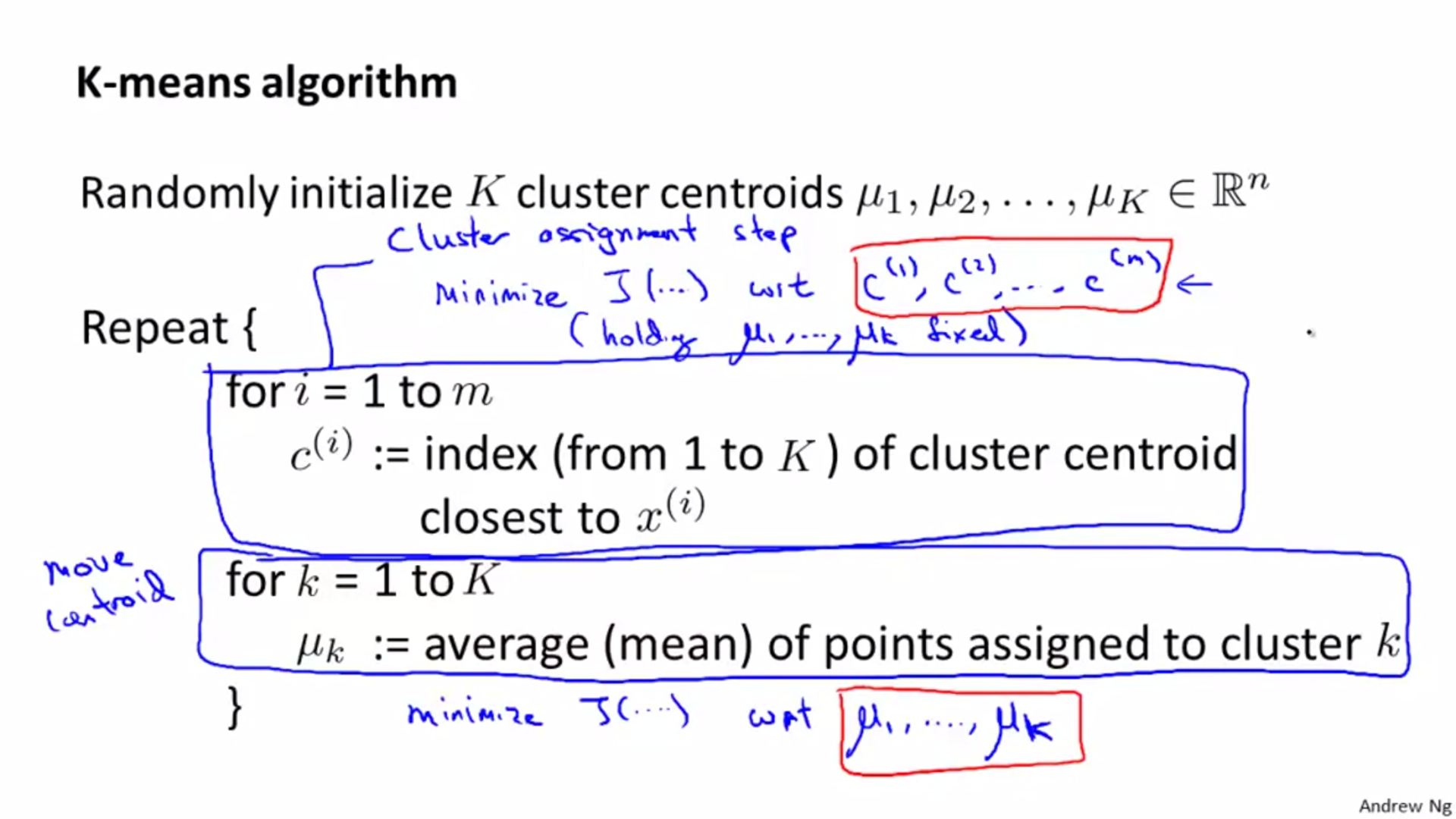
把一些没有加标签的簇分成两类,K-means的步骤如下:
input: K which is the number of clusters;
training set: x(1), x(2), x(3)... x(m)
首先随机选两个点作为簇中心,K-Means主要用于簇分配和移动聚类中心;
根据到簇中心的距离,将dataset分为两类/若干类;
移动聚类中心,继续做上述dataset到簇中心距离的计算;
这个循环做到直到dataset分类不再变化为止;
8.2Optimization
K-means optimization objective
c(i) = index of cluster (1,2,...,k) to which example x(i) is currently assigned; 聚类索引
u(k) = cluster centroid k; 聚类中心
u_c(i) is cluster centroid of cluster to which example x(i) has been assigned 聚类的聚类索引,比如有多个聚类,通过c(i)可以索引到不同聚类中心
8.2Motivation
8.2.1data compression
for data compression, it is known that 3d to 2d and 2d to 1d.
for a dataset of examples{x(1),x(2),x(3),...,x(m)}, x(i) is belonging to Rn, so if we get a lower dimensional dataset{z(1),z(2),z(3),...,z(m)} of examples, z(i) is belonging to Rk for some value of k and k<n. it is called data compression.

8.2.2visualization
in the field of visualization, we can see the figure of lower dimensionality such as 3d or 2d, but we don't have ways to visualize higher dimensional data.
8.3Principal component analysis(PCA)
PCA用于压缩特征,提高算法速度,降低过拟合的风险
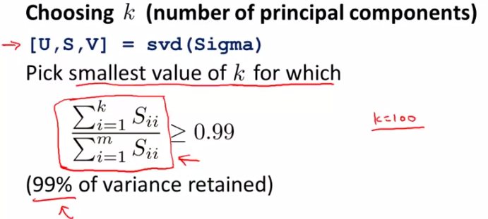
8.3.1选择k的数量
k is the number of PCA
average squared projection error平均平方映射误差
total variation in the data数据总变差


PCA算法的作用是选取最小的满足式子的k值(平均平方映射误差/数据总变差满足大于99%剩余方差)
8.3.2应用PCA
什么时候使用PCA算法:当原始数据过大,导致数据量大,计算速度慢,占用内粗过多时,考虑使用pca算法
8.3.3homework
week09Anomaly detection(异常检验)
9.1异常检验算法
9.1.1density estimation
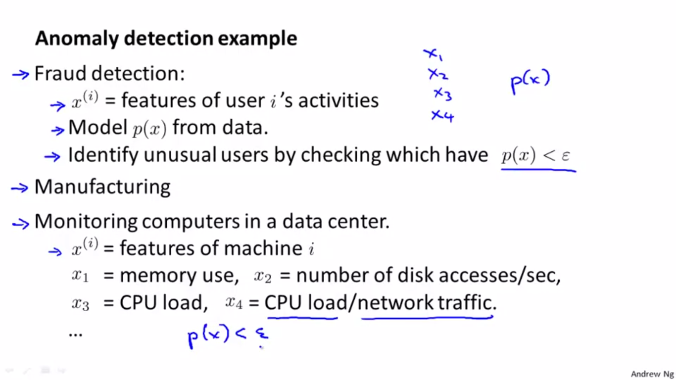
首先设置absilong值,在absilong值内部,被视为合格,非异常点;在absilong外部,被视为异常点。
正常情况下,需要建立模型探测物体(比如计算机)
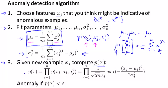
9.1.2algorithm of anomaly detection
解决异常方法,从数据中建立一个p(x)概率模型,用连乘符号来表示估计密度。
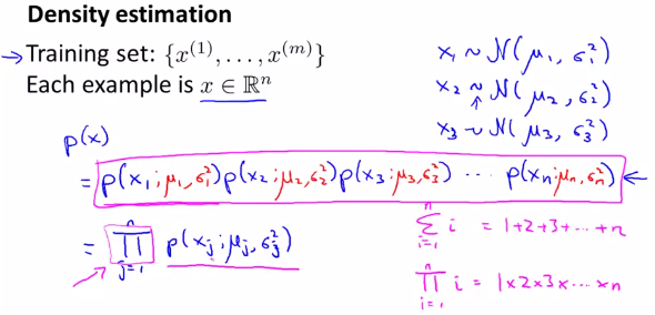
异常检测算法
数据拟合p(x)=p(x1,u1,sigma1^2)*p(x2,u2,sigma2^2)
9.2Building an anomaly detection system
9.2.1developing and evaluating an anomaly detection system
一般情况下如果有10000个examples,那么可以设置training examples = 6000, cross validation examples = 2000, testing examples = 2000
algorithm evaluation

评价异常检验算法的准确性,用F1积分值判断;F1积分值用真值表来确定,还有true positive,false positive,true negative,false negative,recall,accuracy等参数都可以确定下来。
9.2.2anomaly detection vs. supervised learning
异常探测学习对比监督学习
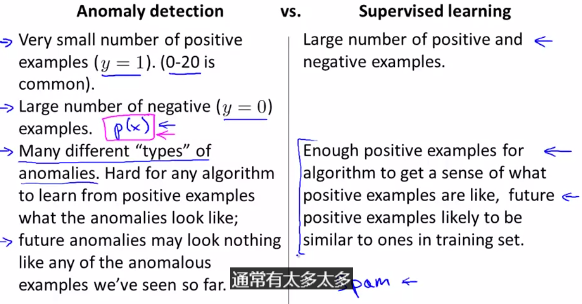
异常探测是小样本的,存在大量负样本的,未来样本预测性不强的,样本具有多样性的;
监督学习是大量数据集的,正负样本数量基本一致的,未来样本预测性强。
异常探测与监督学习的对比(应用方面)
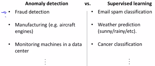
异常检测:反欺诈检测,航空制造业,在数据中心检测数据;
监督学习:垃圾邮件分类,天气预测,癌症判断(是否患癌症)。
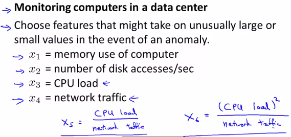
9.2.3choosing what features to use
sometimes, the algorithm is performing poorly, so adding more features to the function is a good method.
9.3multivariate gaussian distribution
9.3.1multivariate gaussian distribution
多元高斯正态分布,改良版的异常检测算法
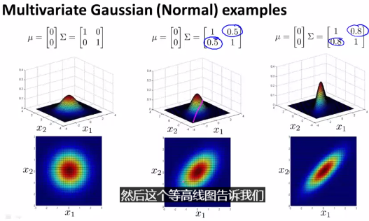
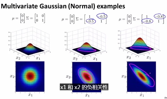
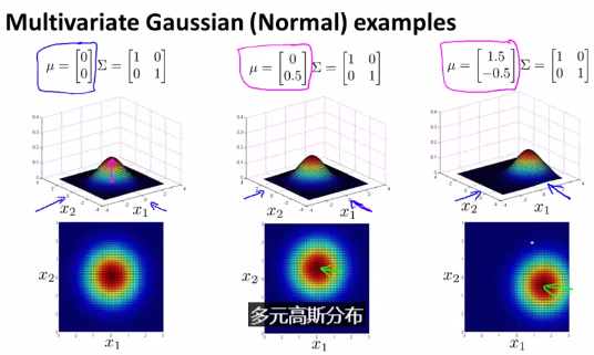
有两种情况,两个参数u和sigma;
u就是左右横移,sigma就是扩展和压缩;
sigma伸张情况
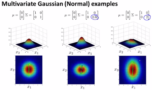
sigma收缩情况
u横移,sigma收缩情况
9.3.2Anomaly Detection using the Multivariate Gaussian Distribution
匹配模型的两个步骤
首先,匹配模型p(x)通过设置u和sigma
其次给出一个新的样例x,计算p(x)

多元高斯分布有两个功能:
1.自动捕捉特征之间的正相关和负相关;
2.标记不正常的特征。
9.4predicting movie ratings
9.4.1Content Based Recommendations
问题描述的参数定义
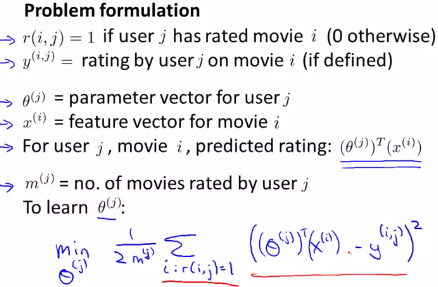
给予内容的推荐,给予内容的假设
9.4.2Collaborative Filtering
推荐机系统recommender systems
协同过滤collaborative filting
协同过滤算法执行场合:当执行协同过滤算法时候,通过一大堆用户得到的数据,这些用户实际上在高效地进行了协同合作,来得到每个人对电影的评分值。只要用户对某几部电影进行评分,每个用户就都在帮助算法,更好地学习出特征,这样,通过自己对几部电影评分以后,就能帮助系统更好地学习到特征,被系统运用,为其他人做出更准确的电影预测;每位用户都在为大家的利益,学习出更好的特征。
9.4.3Collaborative Filtering Algorithm
协同过滤算法对象,这里把两组参数整合成一组数据
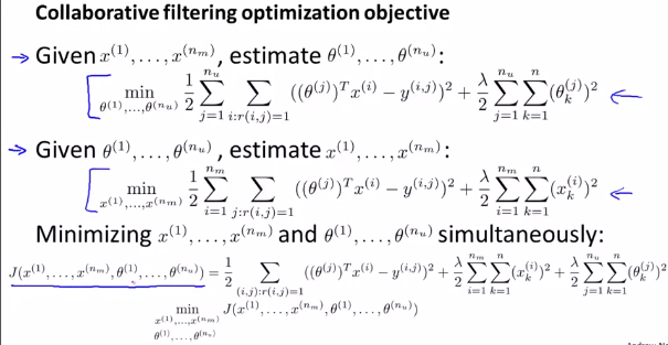
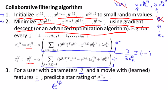
协同过滤算法步骤
第一步初始化X向量和theta向量到小的随机值;
第二步减小J值,使用梯度算法或者高级优化算法;
第三步带有参数theta的用户和带有特征x的电影,预测星级,thetaT*x的排名
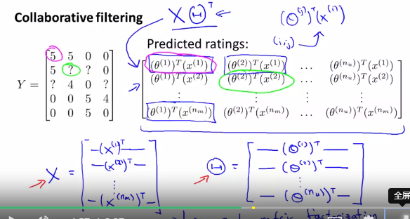
9.5Vectorization: Low Rank Matrix Factorization
预测排名算法 predict rating = X * theta', when x and theta are below
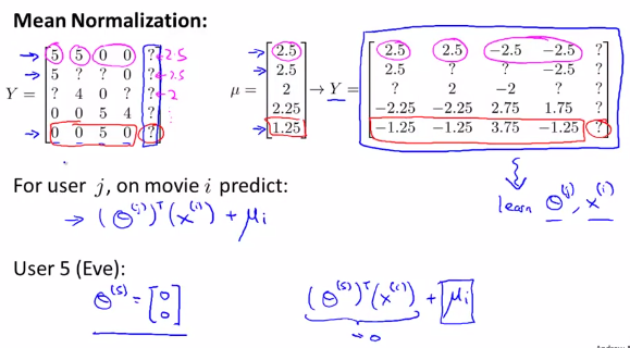
9.5.1Implementational Detail: Mean Normalization
recommender system,均值归一化,
均值归一化后得到的theta(5)的值
9.6homework


 浙公网安备 33010602011771号