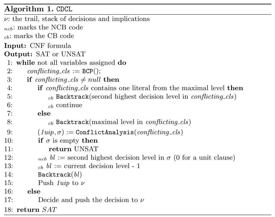
1.先给出最新的回溯方法代码——NCB+CB组合;
2.随后给出文献

所述的CB方法。
3.最后给出CB方法的透彻理解相关代码解读
第一部分:最新求解器均采用的时序回溯组合非时序回溯方法代码
1             ConflictData data = FindConflictLevel(confl);
2
3             if (data.nHighestLevel == 0) return l_False;
4
5             if (data.bOnlyOneLitFromHighest)
6             {
7                cancelUntil(data.nHighestLevel - 1);
8                continue;
9             }
|
|
1 inline Solver::ConflictData Solver::FindConflictLevel(CRef cind) 2 { 3 ConflictData data; 4 Clause& conflCls = ca[cind]; 5 data.nHighestLevel = level(var(conflCls[0])); 6 if (data.nHighestLevel == decisionLevel() && level(var(conflCls[1])) == decisionLevel()) 7 { 8 return data; 9 } 10 11 int highestId = 0; 12 data.bOnlyOneLitFromHighest = true; 13 // find the largest decision level in the clause 14 for (int nLitId = 1; nLitId < conflCls.size(); ++nLitId) 15 { 16 int nLevel = level(var(conflCls[nLitId])); 17 if (nLevel > data.nHighestLevel) 18 { 19 highestId = nLitId; 20 data.nHighestLevel = nLevel; 21 data.bOnlyOneLitFromHighest = true; 22 } 23 else if (nLevel == data.nHighestLevel && data.bOnlyOneLitFromHighest == true) 24 { 25 data.bOnlyOneLitFromHighest = false; 26 } 27 } 28 29 if (highestId != 0) 30 { 31 std::swap(conflCls[0], conflCls[highestId]); 32 if (highestId > 1) 33 { 34 OccLists<Lit, vec<Watcher>, WatcherDeleted>& ws
|
|
| 以上两段代码比较容易理解。 | |
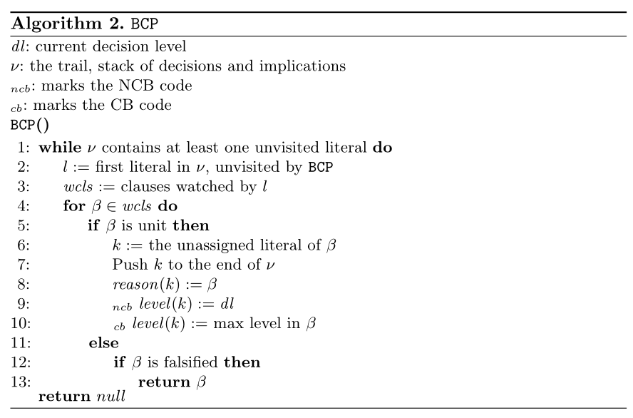
1 CRef Solver::propagate() 2 { 3 CRef confl = CRef_Undef; 4 int num_props = 0; 5 watches.cleanAll(); 6 watches_bin.cleanAll(); 7 8 while (qhead < trail.size()){ 9 Lit p = trail[qhead++]; // 'p' is enqueued fact to propagate. 10 int currLevel = level(var(p)); 11 vec<Watcher>& ws = watches[p]; 12 Watcher *i, *j, *end; 13 num_props++; 14 15 vec<Watcher>& ws_bin = watches_bin[p]; // Propagate binary clauses first. 16 for (int k = 0; k < ws_bin.size(); k++){ 17 Lit the_other = ws_bin[k].blocker; 18 if (value(the_other) == l_False){ 19 confl = ws_bin[k].cref; 20 #ifdef LOOSE_PROP_STAT 21 return confl; 22 #else 23 goto ExitProp; 24 #endif 25 }else if(value(the_other) == l_Undef) 26 { 27 uncheckedEnqueue(the_other, currLevel, ws_bin[k].cref); 28 29 #ifdef PRINT_OUT 30 std::cout << "i " << the_other << " l " << currLevel << "\n"; 31 #endif 32 } 33 } 34 35 for (i = j = (Watcher*)ws, end = i + ws.size(); i != end;){ 36 // Try to avoid inspecting the clause: 37 Lit blocker = i->blocker; 38 if (value(blocker) == l_True){ 39 *j++ = *i++; continue; } 40 41 // Make sure the false literal is data[1]: 42 CRef cr = i->cref; 43 Clause& c = ca[cr]; 44 Lit false_lit = ~p; 45 if (c[0] == false_lit) 46 c[0] = c[1], c[1] = false_lit; 47 assert(c[1] == false_lit); 48 i++; 49 50 // If 0th watch is true, then clause is already satisfied. 51 Lit first = c[0]; 52 Watcher w = Watcher(cr, first); 53 if (first != blocker && value(first) == l_True){ 54 *j++ = w; continue; } 55 56 // Look for new watch: 57 for (int k = 2; k < c.size(); k++) 58 if (value(c[k]) != l_False){ 59 c[1] = c[k]; c[k] = false_lit; 60 watches[~c[1]].push(w); 61 goto NextClause; } 62 63 // Did not find watch -- clause is unit under assignment: 64 *j++ = w; 65 if (value(first) == l_False){ 66 confl = cr; 67 qhead = trail.size(); 68 // Copy the remaining watches: 69 while (i < end) 70 *j++ = *i++; 71 }else 72 { 73 if (currLevel == decisionLevel()) 74 { 75 uncheckedEnqueue(first, currLevel, cr); 76 77 #ifdef PRINT_OUT 78 std::cout << "i " << first << " l " << currLevel << "\n"; 79 #endif 80 } 81 else 82 { 83 int nMaxLevel = currLevel; 84 int nMaxInd = 1; 85 // pass over all the literals in the clause 注意: (1)上述红色标出的代码体现了时序回溯文献所讲的:Unlike in the NCB case, the decision levels of literals in the trail are not necessary monotonically increasing. 也就是说,新进入传播队列的被赋值文字所在层标记号并不一定是与决策层号一致(新近队列文字的层号可能小于本层前次保留的文字所对应的层号——决策层号) (2)对uncheckedqueue函数和传播函数中行81~108代码重点理解并加深认识新进文字的层号。 |
|
2. 加深理解文献:Alexander Nadel, Vadim Ryvchin:Chronological Backtracking. SAT 2018: 111-121
| (1)下面为了说明采取时序回溯以避免盲目回溯掉与冲突无关的已有决策层,给出了很特殊情况的一段论述: | |
|
这种情况,采用通用的非时序回溯,由于vsids决策变元选择机制+相位保持技术机制,会出现回溯后重建传播队列的情况,极端情况重建的传播队列文字可能非常巨大。因此采取时序回溯是必要的。 |
|
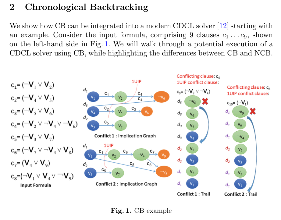
| (2)下面结合实例讲解时序回溯——重点认识确定回溯层和UIP文字反转后加入队列时所对应的层数属性值。 | |
|
|
|
|
|
|
|
(3)CDCL算法
由于传播队列中每层中全体文字各自对应层属性值不同:
需要重点理解两处:传播发生发生冲突后,两处代码做对应处理: 1 ConflictData data = FindConflictLevel(confl); 2 if (data.nHighestLevel == 0) return l_False; //冲突发生在0层,返回结论UNSAT 3 4 if (data.bOnlyOneLitFromHighest) 5 { 6 cancelUntil(data.nHighestLevel - 1);//注意此处回溯到冲突子句文字对应最高层减1 7 continue;//此后由于没有决策文字,BCP无果后会转到无冲突代码段, 1 learnt_clause.clear(); 2 3 if(conflicts > 50000) DISTANCE = 0; 4 else DISTANCE = 1; 5 if(VSIDS && DISTANCE){ 6 collectFirstUIP(confl);} 7 8 analyze(confl, learnt_clause, backtrack_level, lbd); 9 10 // check chrono backtrack condition 11 12 if ( (confl_to_chrono < 0 || confl_to_chrono <= conflicts)
算法流程图:由于line6中continue语句的存在,实际line7~8在真正的solver.cc中并不需要。
说明:1.由于line6中continue语句的存在,实际line7~8在真正的solver.cc中并不需要。 2.line15行是本算法表述对传统CDCL框架表述的明确修正,是本文的亮点。因为以前介绍CDCL的文献,有意无意会漏掉这部分隐含决策变元的加入。
|
|
|
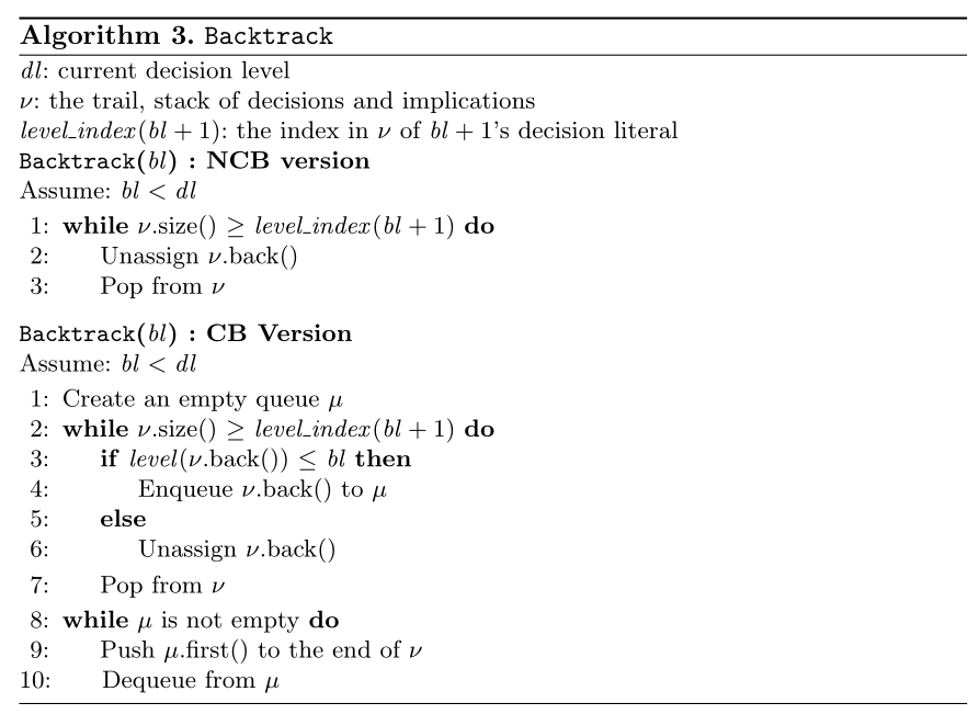
此处的时序回溯中的BCP与Backtrack函数——注意与NCB相应的变化
注:line10只得是当前传播文字l所在reason子句中全体文字对应的最层;由于之前反转文字的加入trail队列,此后传播文字的层号的取值与之前的层号取值就不同了。
BCP operates in a loop as long as there exists at least one unvisited literal in the trail ν. For the first unvisited literal l, BCP goes over all the clauses watched by l. Assume a clause β is visited. If β is a unit clause, that is, all β’s literals are falsified except for one unassigned literal k, BCP pushes k to the trail. After storing k’s implication reason in reason(k), BCP calculates and stores k’s implication level level(k). The implication level calculation comprises the only difference between CB and NCB versions of BCP. The current decision level always serves as the implication level for NCB, while the maximal level in β is the implication level for CB. Note that in CB a literal may be implied not at the current decision level. As usual, BCP returns the falsified conflicting clause, if such is discovered.
注:CB与NCB在回溯的实施中,实际函数void Solver::cancelUntil(int bLevel)没有什么不同,只是对应的实参bLevel不同。
Finally, consider the implementation of Backtrack in Algorithm 3. For the NCB case, given the target decision level bl, Backtrack simply unassigns and pops all the literals from the trail ν, whose decision level is greater than bl. The CB case is different, since literals assigned at different decision levels are interleaved on the trail. When backtracking to decision level bl, Backtrack removes all the literals assigned after bl, but it puts aside all the literals assigned before bl in a queue μ maintaining their relative order. 当回溯到决策层bl时,Backtrack会移除所有赋值在bl之后的字量,但会将赋值在bl之前的字量放在队列μ中,以保持它们的相对顺序。 Afterwards, μ’s literals are returned to the trail in the same order.
|
|
| (3)该文章给出的Combining CB and NCB | |
| 两个阈值C(冲突次数)和T(回溯层跨度)
Our algorithm can easily be modified to heuristically choose whether to use CB or NCB for any given conflict. The decision can be made, for each conflict, in the main function in Algorithm 1 by setting the backtrack level to either the second highest decision level in σ for NCB (line 12) or the previous decision level for CB (line 13). In our implementation, NCB is always applied before C conflicts are recorded since the beginning of the solving process, where C is a user-given threshold. After C conflicts, we apply CB whenever the difference between the CB backtrack level (that is, the previous decision level) and the NCB backtrack level (that is, the second highest decision level in σ) is higher than a user-given threshold T. 下面这段叙述表明,作者认为前期的冲突变元scores需要积累且具有随机性,因此确保C的确定实在随机性被尽可能消除之后;此外作者并没有就回溯门槛的确定T给出具体理由说明。 We introduced the option of delaying CB for C first conflicts, since backtracking chronologically makes sense only after the solver had some time to aggregate variable scores, which are quite random in the beginning. When the scores are random or close to random, the solver is less likely to proceed with the same decisions after NCB. |
|
| (4) 该文章是如何表述实验结果的 | |
|
Experimental Results 3 Experimental Results
3.1 SAT Competition
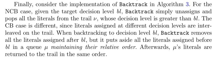
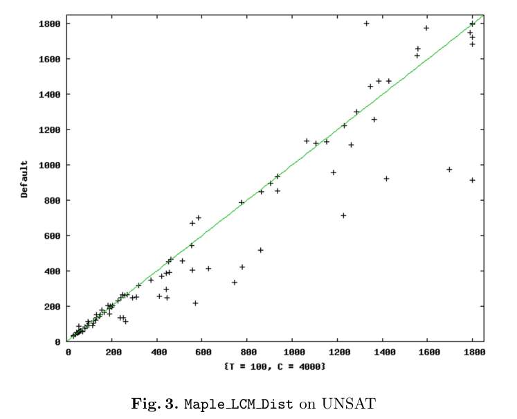
In preliminary experiments, we found that {T = 100, C = 4000} is the best configuration for Maple LCM Dist. Table 1 shows the summary of run time and unsolved instances of the default Maple LCM Dist vs. the best configuration in CB mode, {T = 100, C = 4000}, as well as “neighbor” configurations {T = 100, C = 3000}, {T = 100, C = 5000}, {T = 90, C = 4000} and {T = 110, C = 4000}.
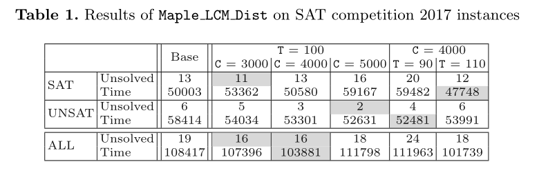
Figure 2 and Fig. 3 compare the default Maple LCM Dist vs. the overall winner {T = 100, C = 4000} on satisfiable and unsatisfiable instances respectively. Several observations are in place.
Several observations are in place. (a1) First, Table 1 shows that {T = 100, C = 4000} outperforms the default Maple LCM Dist in terms of for both the number of solved instances and the run-time. It solves 3 more benchmarks and is faster by 4536 s.
(a2) Second, CB is consistently more effective on unsatisfiable instances. Interestingly,we found that there is one family on which CB consistently yields significantly better results: the 27 instances of the g2-T family. On that family, the run-time in CB mode is never worse than that in NCB mode. In addition, CB helps to solve 4 more benchmarks than the default version and causes the solver to be faster by 1.5 times on average.
(a3) Finally, although the overall winner is slightly outperformed by the default configuration on satisfiable instances, CB can be tuned for satisfiable instances too. {T = 100, C = 3000} solves 2 additional satisfiable instances, whilen {T = 110, C = 4000} solves 1 additional instance faster than the default. We could not pinpoint a family, where CB shows a significant advantage on satisfiable instances. |
|
|
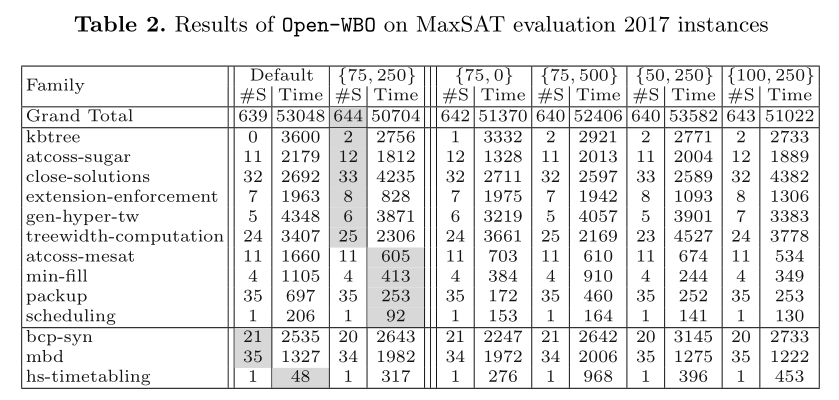
3.2 MaxSAT Evaluation In preliminary experiments, we found that {T = 75, C = 250} is the best configuration for Open-WBO with CB. Consider the five left-most columns of Table 2.
They present the number of solved instances and the run-time of the default Open-WBO vs. {T = 75, C = 250} (abbreviated to {75, 250}) over the MaxSAT Evaluation families (complete unweighted track). (b1) The second row shows the overall results. CB helps Open-WBO to solve 5 more instances in less time.
(b2)
The subsequent rows of Table 2 show the results for families, where either Open-WBO or {T = 75, C = 250} was significantly faster than the other solver, that is, it either solved more instances or was at least two times as fast.
(b3)
One can see that CB significantly improved the performance of Open-WBO on 10 families, while the performance was significantly deteriorated on 3 families only. The other columns of Table 2 present the results of 4 configurations neighbor to {T = 75, C = 250} for reference.
|
|
|
4 Conclusion We have shown how to implement Chronological Backtracking (CB) in a modern SAT solver as an alternative to Non-Chronological Backtracking (NCB), which has been commonly used for over two decades. We have integrated CB into the winner of the SAT Competition 2017, Maple LCM Dist, and the winner of MaxSAT Evaluation 2017 Open-WBO. CB improves the overall performance of both solvers. In addition, Maple LCM Dist becomes consistently faster on unsatisfiable instances, while Open-WBO solves 10 families significantly faster. |
|
|
References
13. Marques Silva, J.P., Sakallah, K.A.: GRASP - a new search algorithm for satisfiability. In: ICCAD, pp. 220–227 (1996)
|
|