深度学习网络架构(二):AlexNet
简介:Alex在2012年提出的Alex网络模型结构将深度学习神经网络推上了热潮,并获得了当年的图像识别大赛冠军,使得CNN网络成为图像分类的核心算法模型.
论文链接:ImageNet Classification with Deep Convolutional Neural Networks(2012)
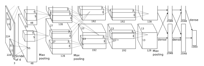
网络结构:AlexNet模型一共有8层,5层卷积层,3层全连接层,在每一个卷积层之后包含Relu激活函数、局部响应归一化、降采样处理,使用2个GPU加速.
- conv1层:
输入:227×227×3,原始彩色图像大小是224×224×3,经过预处理后统一处理为227×227×3的规格
卷积核尺寸:11×11
卷积核个数:96个,2个GPU加速,每个GPU上48个
步长:4
输出:55×55×96 (计算过程:(227-11)/4+1=55 )
激活函数:Relu
降采样处理(pooling):kernel_size=3,stride=2,output=27×27×96(计算过程: (55-3)/2+1=27 )
归一化处理(LRN):local_size=5,output=27×27×96
- conv2层:
输入:27×27×96
填充边界(pad):2
卷积核尺寸:5×5
卷积核个数:256个,2个GPU加速,每个GPU上128个
步长:1
输出:27×27×256 (计算过程:(31-5)/1+1=27 )
激活函数:Relu
降采样处理(pooling):kernel_size=3,stride=2,output=13×13×256(计算过程: (27-3)/2+1=13 )
归一化处理(LRN):local_size=5,output=13×13×256
- conv3层:
输入:13×13×256
填充边界(pad):1
卷积核尺寸:3×3
卷积核个数:384个,2个GPU加速,每个GPU上192个
步长:1
输出:13×13×384 (计算过程:(15-3)/1+1=13 )
激活函数:Relu
降采样处理(pooling):无
归一化处理(LRN):无
- conv4层:
输入:13×13×384
填充边界(pad):1
卷积核尺寸:3×3
卷积核个数:384个,2个GPU加速,每个GPU上192个
步长:1
输出:13×13×384 (计算过程:(15-3)/1+1=13 )
激活函数:Relu
降采样处理(pooling):无
归一化处理(LRN):无
- conv5层:
输入:13×13×384
填充边界(pad):1
卷积核尺寸:3×3
卷积核个数:256个,2个GPU加速,每个GPU上128个
步长:1
输出:13×13×256 (计算过程:(15-3)/1+1=13 )
激活函数:Relu
降采样处理(pooling):kernel_size=3,stride=2,output=6×6×256(计算过程: (13-3)/2+1=6 )
归一化处理(LRN):无
- fc6层:
输入:6×6×256
输出:4096
激活函数:Relu
dropout:0.5
- fc7层:
输入:4096
输出:4096
激活函数:Relu
dropout:0.5
- fc8层:
输入:4096
输出:1000
通过结构可以看出,网络每次都提取出重要的特征,最后通过这些特征确定该图像的类别,抽象之后的结构如下:

创新点:
- Droupout随机权重裁剪:
- 在模型训练过程中,以一定概率随机舍弃某些隐含层节点的权值(认为是0),在更新权值时,不更新与该节点相连的权值.
- 但是被dropout的节点权值得保留下来(只是暂时的不更新),下个样本输入时继续使用该节点权值.
- 减少高激活神经元的数量,提高训练速度,抑制过拟合.
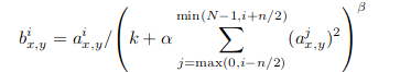
- LRN局部归一化:
- 公式:
![]()
- 提升较大响应,抑制较小响应
- 后来发现效果不明显,所以很少使用.
- 公式:
- MaxPool:
- 避免特征被平均池化模糊,提升特征鲁棒性.
- Relu激活函数:
- 训练中收敛速度更快.
tensorflow代码实现:
  1 from __future__ import print_function
  2 from tensorflow.examples.tutorials.mnist import input_data
  3 import tensorflow as tf
  4 import numpy as np
  5
  6 mnist = input_data.read_data_sets('tmp/data/', one_hot=True)
  7 # MNIST数据集相关常数
  8 input_node = 784
  9 output_node = 10
 10 image_size = 28
 11 num_channel = 1
 12 # 第一层卷积层的尺寸和深度
 13 conv1_deep = 64
 14 conv1_size = 3
 15
 16 # 第二层卷积层的尺寸和深度
 17 conv2_deep = 128
 18 conv2_size = 3
 19
 20 # 第三层卷积层的尺寸和深度
 21 conv3_deep = 256
 22 conv3_size = 3
 23
 24 # 全连接层的节点个数
 25 fc_size = 1024
 26
 27 # 配置神经网络参数
 28 batch_size = 64
 29 learning_rate_base = 0.01
 30 learning_rate_decay = 0.99
 31 training_steps = 10000
 32 moving_average_decay = 0.99
 33
 34 x = tf.placeholder(tf.float32, [None,input_node], name = 'x-input')
 35 y_ = tf.placeholder(tf.float32, [None, output_node], name = 'y-input')
 36
 37 # 定义权重W和偏置b
 38 weights = {
 39     'conv1_weights': tf.Variable(tf.truncated_normal([conv1_size,conv1_size,num_channel,conv1_deep], stddev=0.1)),
 40     'conv2_weights': tf.Variable(tf.truncated_normal([conv2_size,conv2_size,conv1_deep,conv2_deep], stddev=0.1)),
 41     'conv3_weights': tf.Variable(tf.truncated_normal([conv3_size,conv3_size,conv2_deep,conv3_deep], stddev=0.1)),
 42     'fc2_weights': tf.Variable(tf.truncated_normal([fc_size,fc_size], stddev=0.1)),
 43     'out_weights': tf.Variable(tf.truncated_normal([fc_size,output_node], stddev=0.1))
 44 }
 45 biases = {
 46     'conv1_bias': tf.Variable(tf.constant(0.0, shape=[conv1_deep])),
 47     'conv2_bias': tf.Variable(tf.constant(0.0, shape=[conv2_deep])),
 48     'conv3_bias': tf.Variable(tf.constant(0.0, shape=[conv3_deep])),
 49     'fc1_bias': tf.Variable(tf.constant(0.1, shape=[fc_size])),
 50     'fc2_bias': tf.Variable(tf.constant(0.1, shape=[fc_size])),
 51     'out_bias': tf.Variable(tf.constant(0.1, shape=[output_node]))
 52 }
 53 # 定义前向传播model
 54 def cnn(input_tensor):
 55     x_reshape = tf.reshape(input_tensor,shape=[-1,image_size,image_size,num_channel])
 56
 57     conv1 = tf.nn.conv2d(x_reshape,weights['conv1_weights'],strides=[1,1,1,1],padding='SAME')
 58     relu1 = tf.nn.relu(tf.nn.bias_add(conv1,biases['conv1_bias']))
 59     pool1 = tf.nn.max_pool(relu1,ksize=[1,2,2,1],strides=[1,2,2,1],padding='SAME')
 60     norm1 = tf.nn.lrn(pool1,4,bias=1.0,alpha=0.001/9.0,beta=0.75,name='norm1')
 61     norm1 = tf.nn.dropout(norm1,0.8)
 62
 63     conv2 = tf.nn.conv2d(norm1,weights['conv2_weights'],strides=[1,1,1,1],padding='SAME')
 64     relu2 = tf.nn.relu(tf.nn.bias_add(conv2,biases['conv2_bias']))
 65     pool2 = tf.nn.max_pool(relu2,ksize=[1,2,2,1],strides=[1,2,2,1],padding='SAME')
 66     norm2 = tf.nn.lrn(pool2,4,bias=1.0,alpha=0.001/9.0,beta=0.75,name='norm2')
 67     norm2 = tf.nn.dropout(norm2,0.8)
 68
 69     conv3 = tf.nn.conv2d(norm2,weights['conv3_weights'],strides=[1,1,1,1],padding='SAME')
 70     relu3 = tf.nn.relu(tf.nn.bias_add(conv3,biases['conv3_bias']))
 71     pool3 = tf.nn.max_pool(relu3,ksize=[1,2,2,1],strides=[1,2,2,1],padding='SAME')
 72     norm3 = tf.nn.lrn(pool3,4,bias=1.0,alpha=0.001/9.0,beta=0.75,name='norm3')
 73     norm3 = tf.nn.dropout(norm3,0.8)
 74     #print(norm3.shape)
 75
 76     norm3_shape = norm3.get_shape().as_list()
 77     nodes = norm3_shape[1] * norm3_shape[2] * norm3_shape[3]
 78     reshaped = tf.reshape(norm3,[-1,nodes])
 79     #print(reshaped)
 80
 81     fc1_weightst = tf.Variable(tf.truncated_normal([nodes,fc_size], stddev=0.1))
 82     fc1 = tf.nn.relu(tf.matmul(reshaped,fc1_weightst) + biases['fc1_bias'])
 83
 84     fc2 = tf.nn.relu(tf.matmul(fc1,weights['fc2_weights']) + biases['fc2_bias'])
 85
 86     logit = tf.matmul(fc2,weights['out_weights']) + biases['out_bias']
 87     return logit
 88
 89 # 计算前向传播的结果
 90 y = cnn(x)
 91
 92 global_step = tf.Variable(0, trainable=False)
 93 # 初始化滑动平均类,给定训练轮数的变量可以加快训练早期的变量更新速度
 94 variable_averages = tf.train.ExponentialMovingAverage(moving_average_decay, global_step)
 95 # 对所有在神经网络上的参数使用滑动平均,辅助参数不使用(比如global_step)
 96 variables_averages_op = variable_averages.apply(tf.trainable_variables())
 97
 98 cross_entropy = tf.nn.sparse_softmax_cross_entropy_with_logits(logits=y, labels=tf.argmax(y_,1))
 99 loss = tf.reduce_mean(cross_entropy)
100
101 # 设置指数衰减学习率
102 learning_rate = tf.train.exponential_decay(
103     learning_rate_base,global_step,mnist.train.num_examples/batch_size,learning_rate_decay)
104
105 # 开始优化损失函数
106 optimizer = tf.train.GradientDescentOptimizer(learning_rate).minimize(loss)
107 correct_prediction = tf.equal(tf.argmax(y, 1), tf.argmax(y_, 1))
108 # 使用tf.reduce_mean模型将前面的boolean值转换为float值,再求平均值,该值就是准确率
109 accurary = tf.reduce_mean(tf.cast(correct_prediction, tf.float32))
110
111
112 with tf.Session() as sess:
113         # 初始化所有变量
114         tf.global_variables_initializer().run()
115         # 定义测试集
116         test_feed = {
117             x: mnist.test.images,
118             y_: mnist.test.labels
119         }
120
121         for i in range(training_steps):
122             xs, ys = mnist.train.next_batch(batch_size)
123             sess.run(optimizer,feed_dict={x:xs,y_:ys})
124             if i%1000 == 0:
125                 acc = sess.run(accurary,feed_dict={x:xs,y_:ys})
126                 print("After %d training step(s), train accuracy using average model is %g " % (i, acc))
127         test_acc = sess.run(accurary, feed_dict=test_feed)
128         print("After %d training step(s), test accuracy using average model is %g " % (training_steps, test_acc))
运行结果:


 浙公网安备 33010602011771号